
.jpeg)
스팸 필터 관리: 조직을 위한 최적의 필터링 수준 결정
Managing Anti-Spam Filters: Determining the Optimal Level of Filtration for an Organization1
1 뉴브런스윅대학교 세인트존 경영대학 (Faculty of Business, University of New Brunswick Saint John)
*교신저자: 김동민 (dongmin@unb.ca)
DOI: https://doi.org/10.17287/kmr.2026.55.2.555
초록
많은 조직들이 스팸 메일을 탐지하고 격리하기 위해 스팸 필터를 사용하고 있다. 그러나 이러한 필터들은 종종 정상적인 메시지를 스팸으로 오분류하여 통신 지연, 비즈니스 기회 상실, 업무 흐름 방해와 같은 문제를 야기한다. 스팸 통제 실패는 보안상의 허점으로 간주되기 때문에, 관리자들에게 있어 기업의 스팸 필터에 대한 최적의 필터링 수준을 결정하는 것은 중요한 과제이다. 신호 탐지 및 의학 분야에서 수신자 조작 특성(ROC) 곡선과 관련된 유사한 기법들이 논의되어 왔으나, 스팸 필터링을 위한 체계적인 결정 방법은 아직 개발되지 않았다. 본 연구에서는 스팸 필터링 맥락에서 ROC 곡선을 적용하고, 나아가 ROC 곡선을 사용하지 않고도 최적의 임계값을 찾는 새롭고 직접적인 방법을 제안한다. 특정 스팸 필터와 사용자가 인지하는 비용 모델로부터 최적 필터링 수준에 대한 폐쇄형 해(closed-form solution)를 도출하였다. 이러한 최적화 방법은 ROC 곡선이 사용되는 다양한 분야에 적용 가능할 것이다. 연구 결과를 바탕으로 관리자 및 이론적 시사점을 논의한다.
Abstract
Many organizations use anti-spam filters to detect and quarantine unsolicited commercial e-mail. However, these filters often flag legitimate messages as spam, causing problems such as delayed communication, missed business opportunities, and disrupted workflows. Since failure to control spam is often seen as a security lapse, an important question for managers is how to determine the optimal filtration level for a firm’s anti-spam filters. To our knowledge, no systematic way for making such a determination has yet been developed, although analogous techniques relating to the Receiver Operating Characteristic (ROC) curve have been discussed in the signal detection and medical fields. In this regard, we first apply the ROC curve within the context of filtering spam. Furthermore, this research proposes a new and direct method that finds the optimal threshold level without using the ROC curve. A closed-form solution of an optimal filtration level is derived from the model for a given anti-spam filter and a user’s perceived costs. This optimization will be applicable in many areas in which ROC curves are used. Based on the results, implications for managers and implications for theories are discussed.
Ⅰ. Introduction
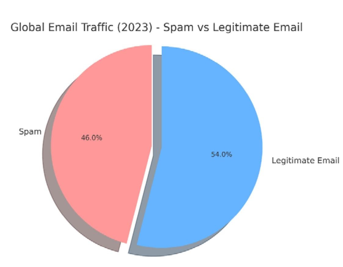
These days, unsolicited commercial email―commonly known as spam―remains a serious issue. As of late 2023 and into 2025, spam makes up roughly 46% of global email traffic, with approximately 160 billion spam messages sent each day (Email ToolTester, 2024; Services, 2024).
The impact goes beyond mere annoyance. Spam drains organizational resources—bandwidth, storage, CPU—and, more critically, employee productivity. Businesses face an estimated annual cost of $20.5 billion due to spam, translating to around $1,934 in lost productivity per employee (Chamaa, 2025).
Many organizations resort to anti-spam filters to fight against spam. Although filters appear to be the best among the anti-spam measures currently available, no perfect filter exists (Pavlov et al., 2005). Imperfect filters inevitably result in two types of undesirable errors: spam that is classified as legitimate e-mail (namely False Negative or FN) and legitimate e-mails that are quarantined as spam (namely False Positive or FP) (Rubenking, 2004; Sun, 2008). Recent advancements, such as large language model (LLM) and AI-based spam filtering, have improved detection accuracy but require substantial computational resources (Alkhdour et al., 2024; Hotoğlu et al., 2025; Roumeliotis et al., 2024; Wang, 2025).
Determining an optimal spam filtration level (or threshold level) for an organization is a challenging decision for managers because of the tradeoff between strengthening and weakening filtering levels. If filtering levels are increased, less spam passes through the filter (i.e., fewer FNs) but more legitimate e-mails are quarantined as spam (i.e., more FPs). Conversely, if filtering levels are decreased, fewer legitimate e-mails are quarantined as spam (i.e., fewer FPs) but more spam gets through the filter (i.e., more FNs).
To date, most research regarding anti-spam filters has focused on filtering algorithms per se (I. Androutsopoulos et al., 2000; M. Sahami et al., 1998; V. Zorkadis et al., 2005) and user behaviors of spam filter apps (Lee & Kwak, 2021). Little research, if any, has been devoted to examining how an organization should set the optimal filtration level for a given anti-spam filter. In this paper, we intend to suggest a systematic way to determine the optimal filtration level for an organization for a given filter.
This situation is similar to the analysis of RADAR signal detection in the 1950s and also to the analysis of medical decisions (for accuracy and comparison of test methods). In such contexts, the Receiver Operating Characteristic (ROC) curve or analysis has been widely applied (Hand, 2009; Krzanowski & Hand, 2009). The ROC curve depicts the True Positive Fraction (TPF) with respect to the False Positive Fraction (FPF). The FPF increases in the TPF, which in turn decreases the False Negative Fraction (FNF), because TPF is defined as 1 minus FNF. Thus, the lower the FNF in the ROC curve, the higher FPF in it. Thus, the dilemma for managers is where to set the appropriate threshold value for spam filtration.
In the first part of this study, in pursuit of our goal, we use the ROC curve-based method because some research in other fields has pursued the use of the ROC curve to set optimal threshold (or classifier) levels in general, and we think this research is applicable to the context of spam filtering as well. The optimization methods includes a maximization of TPF or TNF with given constraints (Mozer et al., 2002), a maximization of accuracy (Fawcett & Provost, 1997; Hanley & Mc Neil, 1982; Hong, 2009), a analytical method using convex hull (Fawcett, 2006; Srinivasan, 1999), a multiple classifier model (Hand et al., 2001) and a cost/benefit analysis using the marginal costs of FN and FP (Metz, 1978).
In the second part of this study, we propose a new model to overcome what we see as a weakness of this ROC-based method. This weakness arises because the ROC-based method can only be used after depicting the ROC curve and then intervening manually to find a touch point between the ROC curve and an optimal line. This manual step is considered a significant barrier for managers to actually implement the ROC-based method. For example, with the ROC-based method, managers need to manually find a tangent point whenever the ROC curve changes due to the environmental changes (i.e., changes in the distribution of Spam and in that of legitimate e-mails). Because the distribution of Spam and that of legitimate e-mails change frequently, it is not feasible or too time-consuming for managers to track the changes and to recalculate the optimal filtering level. In short, the ROC-based method, though theoretically sound, is not a feasible and practical way to find the optimal filtration level for managers. To overcome this weakness of the ROC-based method, we propose a more direct and insightful solution that does not require manual intervention in calculating the optimal filtration level. This new model is important because it can be a basis to automate managers' decisions for the optimal filtration level. If this model is programmed, then the optimal filtration level can be adjusted according to the changes in the environment to meet managers' initial decisions unless managers' initial assumptions (e.g., relative cost of FN and FP in their organizations) change.
We also provide a sensitivity analysis for this new model as a guide in changing parameter values. Then we generalize this solution to double-thresholds values.
To the best of our knowledge, this is the first research that applies the ROC curve within the context of filtering spam. More importantly, this research proposes a new and direct method that finds the optimal threshold level without using the ROC curve.
We think that the implication of the new method is significant because it is applicable in numerous situations in which the ROC curve works, such as signal detection, clinical research, machine learning, etc. The rest of this paper is organized as follows: The literature on spam and the ROC is reviewed in the next section. Subsequent sections contain the model description, solution, sensitivity analysis, and numerical experiment. Lastly, we discuss the implications of our research and our conclusions.
Ⅱ. Literature Review
2.1 Spam Literature
Unsolicited commercial email, commonly referred to as spam, remains a significant vector for cybercrime. While the U.S. Federal Trade Commission (FTC) identified spoofing—the use of falsified email headers—and phishing—fraudulent messages luring users to malicious websites—as primary mechanisms in its 2007 Spam Summit (FTC, 2007), these tactics continue to dominate contemporary spam campaigns. Modern operations are frequently delivered through large-scale botnets, which obscure the sender’s origin and enable mass distribution. Recent telemetry indicates that spam still constitutes approximately 45–47% of global email traffic (2023–2024 averages), with seasonal peaks nearing 49% (Kaspersky, 2025). Botnet command-and-control (C2) infrastructure remains pervasive, with only modest declines in global C2 activity observed in 2024, and regional hosting patterns confirming their ongoing role in spam distribution and malware delivery (Spamhaus Project, 2025).
The thematic composition of spam has evolved only marginally from historical patterns. The dominant categories remain health and medicine, adult content, education and training, IT and technology products, and personal finance; however, recent evidence points to an increasing emphasis on credential theft and payment fraud. In 2024 alone, Kaspersky reported blocking 893 million phishing attempts, representing a 26% year-over-year increase, with these familiar topic clusters continuing to serve as common lures (Kaspersky, 2025). Phishing is also a critical initial access vector in broader cyber incidents—appearing alongside social engineering and credential misuse—factors collectively referred to as the “human element” in approximately 68% of documented breaches (Verizon, 2024).
From a regulatory perspective, both the United States and Canada have established frameworks to address the spam problem. In the United States, the Controlling the Assault of Non-Solicited Pornography and Marketing Act (CAN-SPAM), in effect since January 2004 (FTC, 2023), continues to mandate accurate header information, prohibit deceptive subject lines, and require a functional opt-out mechanism. The framework has remained unchanged, with ongoing enforcement actions by the FTC and partner agencies. In Canada, the anti-spam regime shifted significantly with the implementation of the Canadian Anti-Spam Legislation (CASL) on July 1, 2014 (ISEDC, 2024). CASL prohibits sending commercial electronic messages (CEMs) without prior consent, requires sender identification and an operational unsubscribe mechanism, and extends to malware installation without consent. Enforcement responsibilities are shared among the Canadian Radio-television and Telecommunications Commission (CRTC), the Competition Bureau, and the Office of the Privacy Commissioner. Between 2023 and 2024, Innovation, Science and Economic Development Canada (ISED) reported over $3.2 million in administrative penalties, underscoring the law’s active application and replacing earlier Canadian legal frameworks that tolerated unsolicited commercial email provided headers were not falsified (ISEDC, 2024). Currently, many anti-spam filters are available for free or for purchase. In addition to the anti-spam filters used by organizations, anti-spam filters also are included in public e-mail or Web-based e-mail systems, such as Gmail, Hotmail, and Yahoo! Mail.
Unlike the present study that focuses on an optimal filtration level when a filter (or an algorithm) is given, most research on spam filters has focused on the algorithms per se that detect spam messages by using intelligent filtering (such as a Bayesian filter), the blocking of blacklists, and the allowing of only specific senders. The principal criterion for judging successful filtering algorithms has been filtration power (i.e., percentages of correct filtration out of the total emails), without any differentiation between FP and FN (Androutsopoulos et al., 2000) (I. Androutsopoulos et al., 2000; Sahami et al., 1998; Zorkadis et al., 2005). The concepts of FP and FN have been used in several studies (Androutsopoulos et al., 2000; I. Androutsopoulos et al., 2000; Hong & Cho, 2009; Park et al., 2020; Sahami et al., 1998; Zorkadis et al., 2005), but they considered the economic values of FP and FN as equal. A few studies, however, have discussed the need to assign different values to FP and FN (Cavusoglu et al., 2005; González-Talaván, 2006; Gray & Haahr, 2005; Pelletier et al., 2004; Sun, 2008). For example, Lueg (2005) emphasized the importance of FP in anti-spam filters. Several other articles warned of the critical aspect of FPs and suggested several tips to minimize them (Keizer, 2005; Shavelson, 1996). Cavusoglu et al. (2005) applied FP and FN to examine the value of Intrusion Detection Systems (IDS), where their approach was to find the optimal point in the simultaneous game between IDS and hackers. In extending this field of research, we assume that the values of FPs and FNs can be unequal and can differ from one organization to another. From a user’s viewpoint, the perceived costs of using an anti-spam filter consist of two elements: the cost of deleting FNs from an inbox and the cost of recovering FPs from a quarantined spam box. We will find the most beneficial, or the optimal filtration level for a given anti-spam filter, so as to minimize the perceived total cost.
2.2 ROC Literature
The ROC (Receiver Operating Characteristics; it was originated from use of this curve in Signal Detection Theory) is one of the widely used approaches to evaluate performance of classification systems, where classification results in FP and FN (Krzanowski & Hand, 2009). ROC can be used in various areas, such as medical diagnostics to classify a patient to a certain disease, speech recognition to classify spoken words, financial credit card processing to classify a credit card transaction to a potentially fraudulent one, and so on (Hand, 2009; Krzanowski & Hand, 2009).
While ROC is relatively new to Information Systems researchers, it is one of the popular topics of research and this is evident in over four thousand articles that included either "Receiver Operation Characteristics" or "ROC curves" between 2004 and 2007, according to Krzanowski and Hand (2009) and Hand (2009). While there are many subareas of ROC curve related research, which include comparison of two classification systems (e.g., visual comparison among medical tests and quantitative comparison among medical tests), visual agreement of test accuracy, selection of decision threshold, etc. (Zweig & Campbell, 1993), the present study focuses on selection of decision threshold of ROC and proposes a new model in that area.
The concepts of FP and FN are used in clinical research – especially in psychology and radiology. Sensitivity is the probability of a positive test result among patients with a disease (in our case it is the rate of the correct screening out of spam messages, i.e., "$\alpha$," is the same as TPF – True Positive Fraction), and specificity is the probability of a negative test result among patients without a disease (in our case the rate correctly unscreened, i.e., "1 – $\beta$," is the same as the TNF – True Negative Fraction), as shown in Kwon and Farrell (2000)). Most of the research explains the meaning of sensitivity and specificity in the specific application, and shows how to obtain the ROC curve (Swets, 1988; van Erkel & Pattynama, 1998; Zou et al., 2007; Zweig & Campbell, 1993).
Metz (1978) explained the methodology of using averaging to obtain an optimal threshold. Fawcett and Provost (1997) explored the heuristic fraud detection algorithm using a data mining technique with economic value, although they did not use the ROC curve explicitly. There is also some research extending the optimal condition to n-dimensional ROC space (Hand & Robert, 2001; Srinivasan, 1999). Hong (2009) applied this ROC optimization concept to credit rating in a lending institution. Some research also is available on the statistical or mathematical interpretation of the ROC curve: goodness-of-fit with a distribution assumption (using $\chi^2$ analysis), a non-parametric goodness-of-fit test (Hanley & Mc Neil, 1982), and the meaning of the Area Under Curve (AUC) (Hand, 2009).
Ⅲ. Model Description
3.1 Assumptions and Symbols
We assume that a one-dimensional index, "spam score", is available for incoming e-mails. Depending on the filtration power of the anti-spam filter, the distance between the average legitimate e-mail index and the average spam index varies. The following are several additional assumptions and symbols used in our mathematical formula.
1) Both indices for legitimate e-mail (hereafter designated by the subscript $D^-$) and spam (designated by the subscript $D^+$) are unimodal. Let us assume the mode in $D^-$ less than the mode in $D^+$; or the higher the index score is, the more likely the e-mail is spam.
2) δ is the proportion of spam mail out of all incoming mail (0 ≤ δ ≤ 1).
3) Two types of perceived costs are incurred: CFN is the cost to manually delete one FN message from a user’s inbox, and CFP is the cost to recover one FP from a spam box. The latter includes the opportunity cost of failing to respond to a (quarantined) e-mail on time, the time lost in accessing the spam box, and the cost of an unrecovered legitimate mail.
4) α is the proportion of spam mail classified as spam out of all spam mail received by a given anti-spam filter, or TPF; in other words, 1 - α is the FNF.
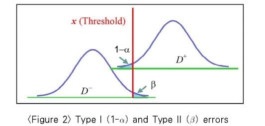
5) β is the proportion of legitimate mail classified as spam out of all legitimate mail received by a given anti-spam filter, in other words, the FPF. β (or a type II error) depends on the distribution and the threshold value defined by 1 - α (that is, a type I error). This is depicted in Figure 2.
3.2 ROC curve
Let D be the disease in question - in our context, the spam - and let T be the test result of a diagnosis, or spam filtration. And we use superscript “+” or “-” for positive and negative, respectively. TPF is $P(T^+/D^+)$ or $P(T^+ \cap D^+)/P(D^+)$, and FPF is $P(T^+/D^-)$ $P(T^+ \cap D^-)/P(D^-)$. The possible contingency table is shown as Figure 3 (a), and the relationship between TPF and FPF is drawn in Figure 3 (b).
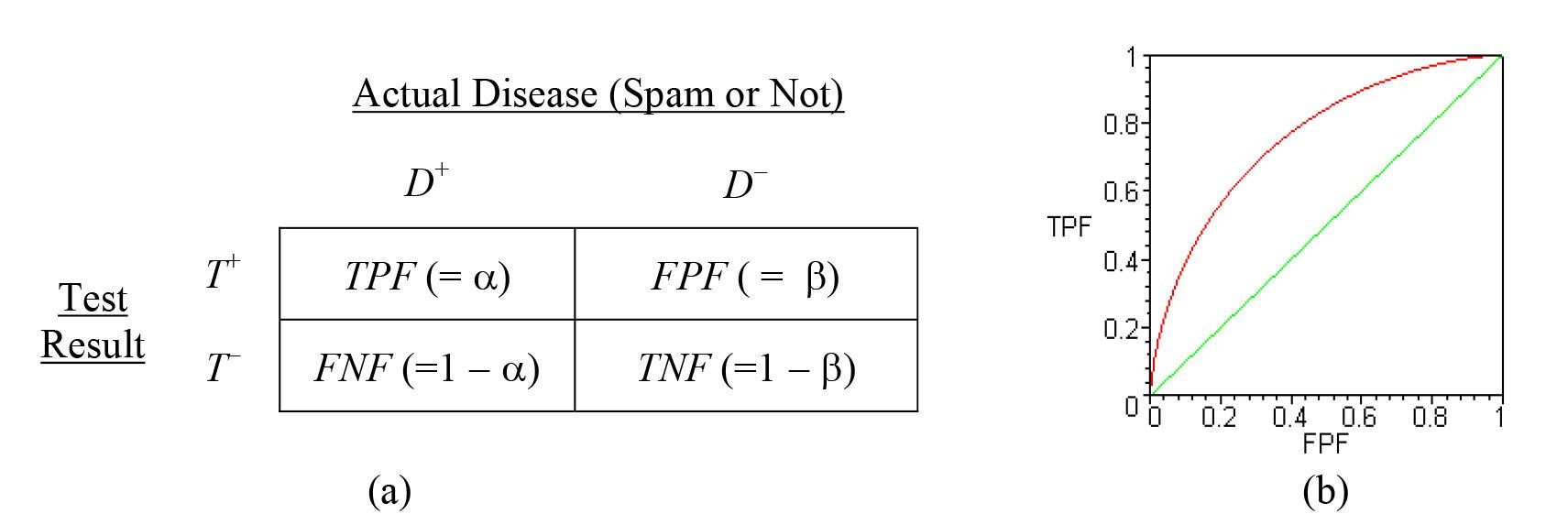
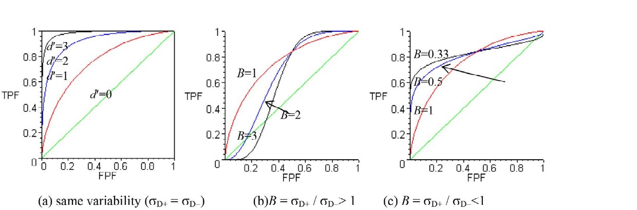
As the ROC curve moves toward the top left corner, the distance of the mean (relative to the standard deviation) between $D^+$ and $D^-$ increases. This distance is the strength of the signal, and it is called the discriminability index ($d'$). The shape is symmetrical for the diagonal line from (0, 1) and (1, 0) if the distribution of $D^+$ and that of $D^-$ have the same variance, as assumed in most signal detection theories. However, when the variances of the two distributions are unequal, the shape is distorted. The difference with $d'$ and variability are shown in Figure 4.
Ⅳ. Optimal Threshold
4.1 Optimization using ROC curve
From the above parameters, we can formulate the average cost for FP and FN. Our objective is to minimize the average cost of the consequences of a spam filter, say $\bar{C}$. Since $P(D^+) = \delta$ and $P(D^-) = 1 - \delta$,
By differentiating with respect to FPF (which is the x-axis in ROC curve), we have
From the First Order Condition (FOC), we have the optimality condition as follows:
If we define $K = \frac{(1-\delta)C_{FP}}{\delta C_{FN}}$, the ratio between the cost incurred from the FP and the cost to manually delete the FN, it is optimal at the point at which the slope of the ROC curve equals $K$. Note that this result is same to the cost/benefit analysis of ROC curve (Metz 1978). However, if $B = \frac{\sigma_{D+}}{\sigma_{D-}} \neq 1$ (the variability differs for $D^+$ and $D^-$ curves; refer to Figure 4 (b)), there exist multiple points satisfying the FOC. By differentiating (2) with FPF, we have $\frac{d^2 \bar{C}}{d(FPF)^2} = -\delta C_{FN} \cdot \frac{d^2(TPF)}{d(FPF)^2}$ to be positive in the minimizing point. Thus, the optimal point satisfies FOC and concavity (i.e, negative $\frac{d^2(TPF)}{d(FPF)^2}$) in the ROC curve.
4.2 Optimization using a direct calculation
Let $F_p(\cdot)$ and $f_p(\cdot)$ be the CDF (cumulative distribution function) and PDF (probability density function) of $D^+$. And let $F_n(\cdot)$ and $f_n(\cdot)$ be the CDF and PDF of $D^-$. We assume that $f_p(\cdot)$ and $f_n(\cdot)$ are differentiable for $x \in [0, 100]$ which is the range of the spam score. For a given threshold $x$, $\alpha(x) = P(X_{D+} > x) = 1 - F_p(x)$ and $\beta(x) = P(X_{D-} > x) = 1 - F_n(x)$. Therefore,
where $K$ is same as the right-hand side of equation (3). Let $x^*$ be the optimal filtration level, or $x^* = \arg \min_{x \in [0, 100]} \bar{C}(x)$. Because $C_{FN}$ is a given value for a specific environment, the choice of optimal $x^*$ only depends on
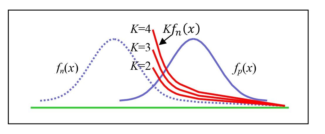
By differentiating and using the first order condition (FOC), we have $C'(x) = f_p(x) - K f_n(x) = 0$ (6). From Figure 5, there would be zero to two points satisfying FOC. Without loss of generality, we assume $K > 1$ because $(1-\delta)C_{FP}$ is greater than $\delta C_{FN}$.
Lemma 1. (Optimal solution for general PDF)
(a) $x^* = 100$ for a large $K$ which has no point satisfying $f_p(x) = K f_n(x)$.
(b) $x^* = \min\{x | f_p(x) = K f_n(x)\}$ for $K$ satisfying FOC for some $x \in [0, 100]$.
Proof. (a) In this case, $f_p(x) < K f_n(x)$ for all $x \in [0, 100]$. Because $C'(x) < 0$, the largest value in the range is optimal. (b) Let’s assume that both $x_1$ and $x_2$ satisfies FOC, and $x_1 \leq x_2$. Then, $C(x + \Delta) - C(x) - \Delta \cdot C'(x) = \int_{x}^{x+\Delta} (f_p(z) - K f_n(z)) dz - K \cdot (F_n(x+\Delta) - F_n(x))$. For $z \in [x_1, x_1 + \Delta]$, $C'(z) = f_p(z) - K f_n(z) > 0$ and the above equation becomes positive, which means $C''(x_1) > 0$ by the definition of convexity. For $z \in [x_1, x_2 + \Delta]$, $C'(z) = f_p(z) - K f_n(z) < 0$ and $C''(x_2) < 0$. Hence, $x_1$ is the minimum point.
In the next section, we find the optimal solution in the normal distribution. From the closed form solution, we will further investigate the sensitivity analysis about the controllable parameters.
4.3 Optimization in Normal Distribution
Both indices for legitimate e-mail (hereafter designated by the subscript $D^-$) and spam (designated by the subscript $D^+$) are normally distributed, i.e., $X_{D^-} \sim N(\mu_{D^-}, \sigma_{D^-})$ and $X_{D^+} \sim N(\mu_{D^+}, \sigma_{D^+})$, respectively. As mentioned, the spam score is higher in spams and thus $\mu_{D^-} \leq \mu_{D^+}$.
Let $\Phi(\cdot)$ and $\phi(\cdot)$ be a standard normal PDF and CDF, respectively. For a given $\alpha (= TPF)$, the cutoff point, $x$, is defined as
and, $\beta (= FPF)$ is calculated from the $D^-$ distribution as follows:
where substituting $A = (\mu_{D^-} - \mu_{D^+}) / \sigma_{D^-}$, $B = \sigma_{D^+} / \sigma_{D^-}$ and $X = \Phi^{-1}(\alpha)$.
Note that $X$ is the $Z$-value for the threshold $x$ from the $D^+$ distribution, and $A + BX$ is the $Z$-value for the cutoff point $x$ from the $D^-$ distribution. Since $\mu_{D^+} \geq \mu_{D^-}$, we always have $A < 0$ and $B > 0$. $A$ is similar to the discriminability index ($d''$) in ROC curve. If $B \neq 1$, the ROC curve is twisting as shown in Figure 4 (b).
From (7), we use $\alpha$, instead of $x$, as our decision variable, hereafter. By substituting (8) into (1), we have the following equation for $C(\alpha)$:
which only contains $A$, $B$, and $K$. Since $\phi'(x) = -x\phi(x)$ for a normal density function $\phi(x)$, we have
Observation 1. (Finding the distribution parameters) From two distinct data sets $(\alpha_1, \beta_1)$ and $(\alpha_2, \beta_2)$, there exist unique parameters $A$ and $B$.
Please refer to the Appendix for all proofs for observations and lemmas.
Lemma 2. (Convexity of curve) If $B = 1, C(\alpha)$ is convex for all $\alpha$. Otherwise, $C(\alpha)$ has only one inflection point at $\alpha = \Phi\left(\frac{AB}{1-B^2}\right)$ and $C(\alpha)$ changes from convex to concave for $B > 1$, and from concave to convex for $B < 1$.
From Lemma 2, there exists a unique solution to minimize the total cost in the convex range. In most cases where $\alpha > 50\%$ (i.e., $f_p'(x) > 0$) and $\beta < 50\%$ (i.e., $f_n'(x) < 0$), the corresponding $C''(\alpha) = f_p'(x) - Kf_n'(x) > 0$ from (6).
Lemma 3. (Optimal solution) Let $D = A^2 - 2(1 - B^2) \ln(BK)$. The optimal solution $\alpha^*$ is as follows: (a) If $B = 1, \alpha^* = \Phi\left(\frac{2 \ln(K) - A^2}{2A}\right)$. (b) If $B \neq 1$ and $D < 0$, then $\alpha^* = 0$ for $B < 1$ and $\alpha^* = 1$ for $B > 1$. (c) If $B \neq 1$ and $D \geq 0$, then there exists a local optimal point $\alpha^* = \Phi\left(\frac{AB + \sqrt{D}}{1 - B^2}\right)$.
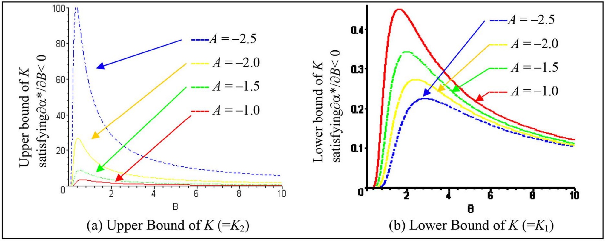
Since we have a closed-form solution for the optimal filtration level, a sensitivity analysis of the solution is possible, as explained in the Lemma 3. $D$ is the inside of root in the optimal solution as shown in part (c). Note that $D < 0$ is an extreme case that rarely happens in which $K < \exp\left(\frac{A^2}{2(1-B^2)}\right)/B$ for $B > 1$ and $K > \exp\left(\frac{A^2}{2(1-B^2)}\right)/B$ for $B < 1$. This is the case of no point satisfying FOC in Lemma 1. At $A = -2.5$, the range for $K$ value for the boundary solution is shown in Figure 6. Note that the optimal $\alpha$ level for $B < 1$ is 0; that is, the optimal solution is to disable the anti-spam filter when $K$ is extremely high. On the other hand, for $B > 1$, the optimal $\alpha$ becomes 1 (in other words, using the full power without worrying about $FP$) when $K$ is extremely low.
These optimal values are intuitively true because if $FP$ were very critical, the user would turn off the anti-spam filter, and if $FP$ were of little value compared to $FN$, the user would fully use the anti-spam filter. But the question is why $\alpha^*$ depends on $B$. Let’s assume a very high $K$ for $B < 1$. From $B = \sigma_{D^+} / \sigma_{D^-}$, the $D^-$ is distributed more widely than $D^+$, and thus, to keep all legitimate e-mails, it is better to turn off the anti-spam filter. On the other hand, for $B > 1$, the $D^+$ are distributed widely and the $D^-$ narrowly, and thus, there would be a possible way to control some of the spam without worrying about $FP$.
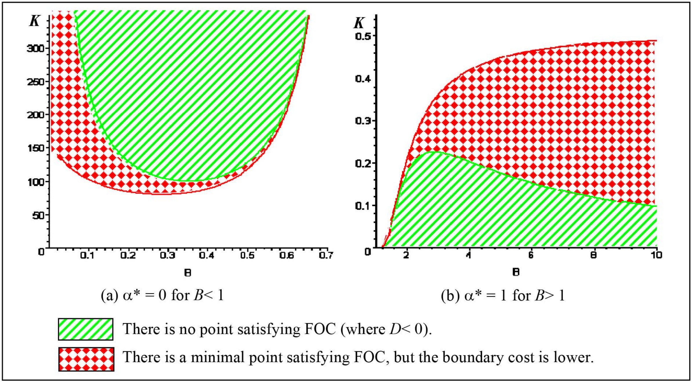
However, the minimal boundary solution can be found in a different range for $B$. Although there is a point satisfying the FOC in the convex range, the real optimal solution is obtained by comparing $\alpha$ with the boundary value, that is, $\alpha = 0$ for $B < 1$ and $\alpha = 1$ for $B > 1$. This is summarized in Figure 7, which shows all possible cases depending on $B$ and $K$. Because the boundary optimal solution is only obtained with extremely high $K$ (for $B < 1$) or extremely low $K$ (for $B > 1$), the $\alpha^*$ in the convex region is a true optimal value under fairly general conditions. Note that the extremely low $K$ is not in our scope.
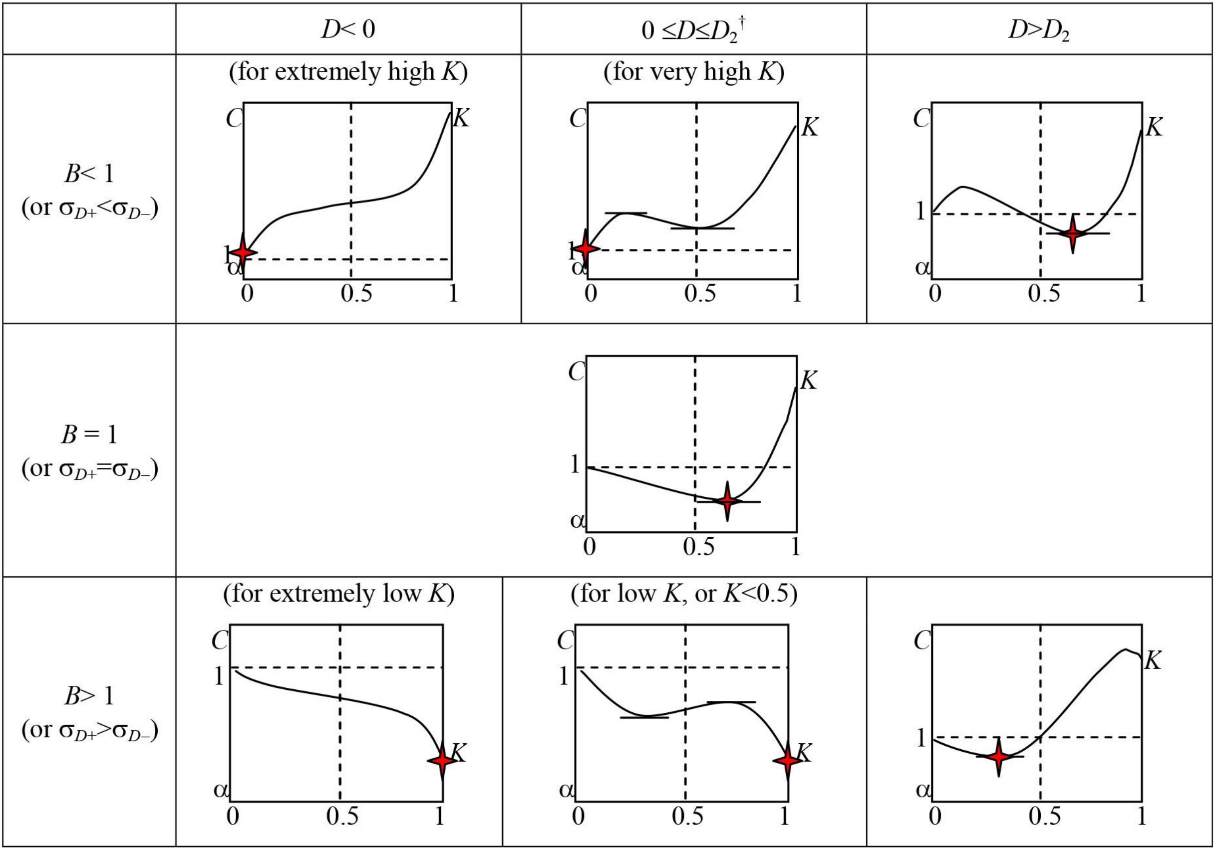
When $\alpha^*$ in the convex region from Lemma 2 (c) is the global optimal for the cost function $C(\alpha)$, we have the following result for a parametric change.
Lemma 4. (Sensitivity analysis of parameters)
(a) $\alpha^*$ is decreasing as $A$ increases.
(b) As $B$ increases, $\alpha^*$ is decreasing if $K < 1/B \exp(-(A\sqrt{A^2+4}(1+B^2)+(A^2+2)(1-B^2))/4B^2)$. Otherwise, $\alpha^*$ increases.
(c) As $K$ increases, $\alpha^*$ decreases.
Since $A = (\mu_{D^+} - \mu_{D^-}) / \sigma_{D^-}$ and $B = \sigma_{D^+} / \sigma_{D^-}$, the spam becomes more intelligent as $A$ and/or $B$ increase. Here, the intelligence of spam is revealed by how difficult it is for the anti-spam filter to differentiate spams from legitimate e-mails. As the filtering percentage increases for intelligent spam, an increase in $FP$ is unavoidable, resulting in an increase in recovery cost for $FP$. For example, unless $K$ is very small, the increase in $FP$ is hard to bear, and the optimal level of $\alpha$ decreases in order to prevent the higher Type-II error as spam becomes smarter than before.
4.4 Optimization for general distributions
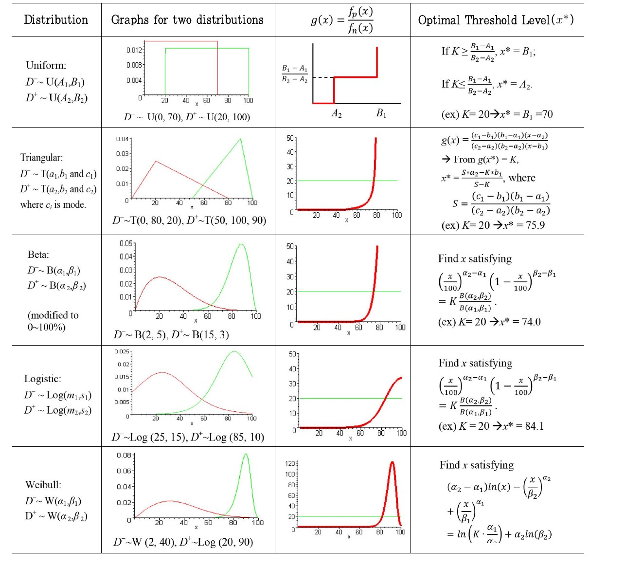
We used a normal distribution to compute the optimal solution and to show the general behavior of the optimality by changing parameters in Lemma 3 and 4. However, there are pitfalls to apply the normal distribution in the spam filtration. First of all, the actual data may not follow the normal distribution – probably data distributions are highly skewed depending on which filters the company or the individual uses. Secondly, the normal distribution has the wider range than our spam score, say, between 0 and 100. The more appropriate analysis is using the truncated distribution, which results in deteriorating the straightforward intuition about the optimality.
From the FOC of (6), we have the optimality condition of $C'(x) = f_p(x) - K f_n(x) = 0$. If we say $g(x) = f_p(x)/f_n(x)$, the optimality condition is $g(x) = K$. Under the condition of continuity and unimodality, we will show briefly how this optimality condition works in different distributions in Table 1.
Table 1 Other distributions and the optimality
4.5 Optimization for multiple-thresholds
To mitigate the extreme effects of $FN$ or $FP$, some filters use double-threshold filtration. Analogous to the double sampling inspection used in the quality control, this system has two threshold values as shown in Figure 8. If the spam score (SS) of a certain e-mail is greater than $M_1$, then it will be filtered out and sent to the spam box. If $M_2 \leq SS < M_1$, the e-mail is delivered into the user’s inbox with a spam-warning prefix in the subject line. When $SS < M_2$, this email is assumed legitimate and is delivered to the inbox without any warning in the subject.
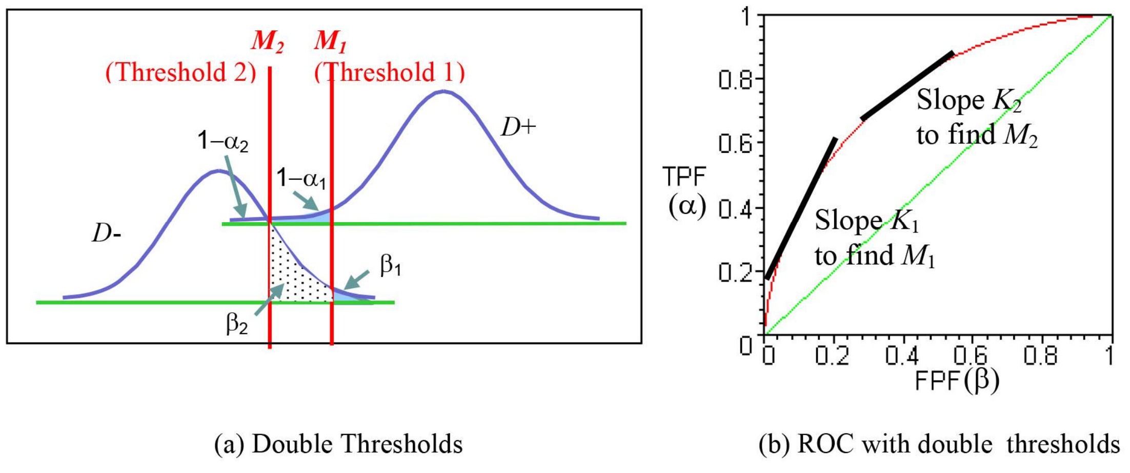
Two types of perceived cost are incurred for $FN$: $C_{FN_2}$ is the cost to manually delete one $FN$ message (without any spam warning) from a user’s inbox; on the other hand, $C_{FN_1}$ is the cost to delete one $FN$ message with a spam warning. Because the latter is noticeable, we assume $C_{FN_2} > C_{FN_1}$. Similarly, there are two different $FP$-related costs: $C_{FP_1}$ is the cost to recover one $FP$ from a spam box (or the cost incurred because one is not delivered), and $C_{FP_2}$ is the cost to check the legitimacy of the message with a spam-warning subject; hence, $C_{FP_2} \ll C_{FP_1}$. In most cases, $C_{FP_1}$ is much higher than $C_{FN_1}$. We use subscripts 1 and 2 for thresholds $M_1$ and $M_2$, respectively. Then, we have an average cost
By differentiating with respect to $FPF_1$ and $FPF_2$, the FOC indicates that the slope is $K_1 = \frac{(1 - \delta)(C_{FP_1} - C_{FP_2})}{\delta C_{FN_1}}$ at the first and $K_2 = \frac{(1 - \delta)C_{FP_2}}{\delta(C_{FN_2} - C_{FN_1})}$ at the second threshold from the ROC curve.
Lemma 5. (Conditions for $K_1 > K_{i+1}$ for all $i = 1, \dots, n$)
(a) If $C_{FP_{i+1}} < \frac{1}{2}(C_{FP_i} + C_{FP_{i+2}})$ and $C_{FN_{i+1}} > \frac{1}{2}(C_{FN_i} + C_{FN_{i+2}})$ for all $i$, then $K_1 > K_{i+1}$.
(b) If $C_{FP_{i+1}} \leq 2C_{FP_i}$ and $C_{FN_{i-1}} \leq 2C_{FN_i}$ for all $i$, then $K_1 > K_{i+1}$.
The proof of Lemma 5 is trivial. If we have $K_1 > K_{i+1}$ for all $i$, it is better off to use $n$ thresholds to reduce the total cost of $FP$’s and $FN$’s. This is the guideline to determine how many thresholds should be used for a spam filtration system.
V. Numerical Experiments
Suppose that the IT department tests an anti-spam filter system and gathers $(\alpha, \beta) = (75\%, 2.2\%)$ for a threshold spam-score (say, SS) of 80 and $(\alpha, \beta) = (63\%, 1.2\%)$ for SS = 85. Since the values for $C_{FP}$ and $C_{FN}$ are relative, the $C_{FP} / C_{FN}$ can be obtained from the question, “If your cost to delete one SPAM mail in your INBOX is 1 cent, what would be your cost of recovering a legitimate mail that is quarantined by the anti-spam filter?” If the answer was 50 cents, then $C_{FP} / C_{FN}$ would be ¢50 / ¢1 = 50. Assume that the percentage of spam, out of all incoming mail, or $\delta$, is 0.891 (taken from MessageLabs data, 2011). Hence, $K = \frac{(1-\delta)C_{FP}}{\delta C_{FN}} = 6.12$. Notice that $K$ changes in $\delta$ dramatically, such as $K = 5.56$ for $\delta = 0.9$, $K = 12.5$ for $\delta = 0.8$ and $K = 21.43$ for $\delta = 0.7$.
Using two points of $(\alpha, \beta)$, we have $(A, B) = (-2.49, 0.71)$ from Observation 1. We have
where $\alpha = \Phi(X)$. The shape of $C(\alpha)$ is shown in Figure 9 (a).
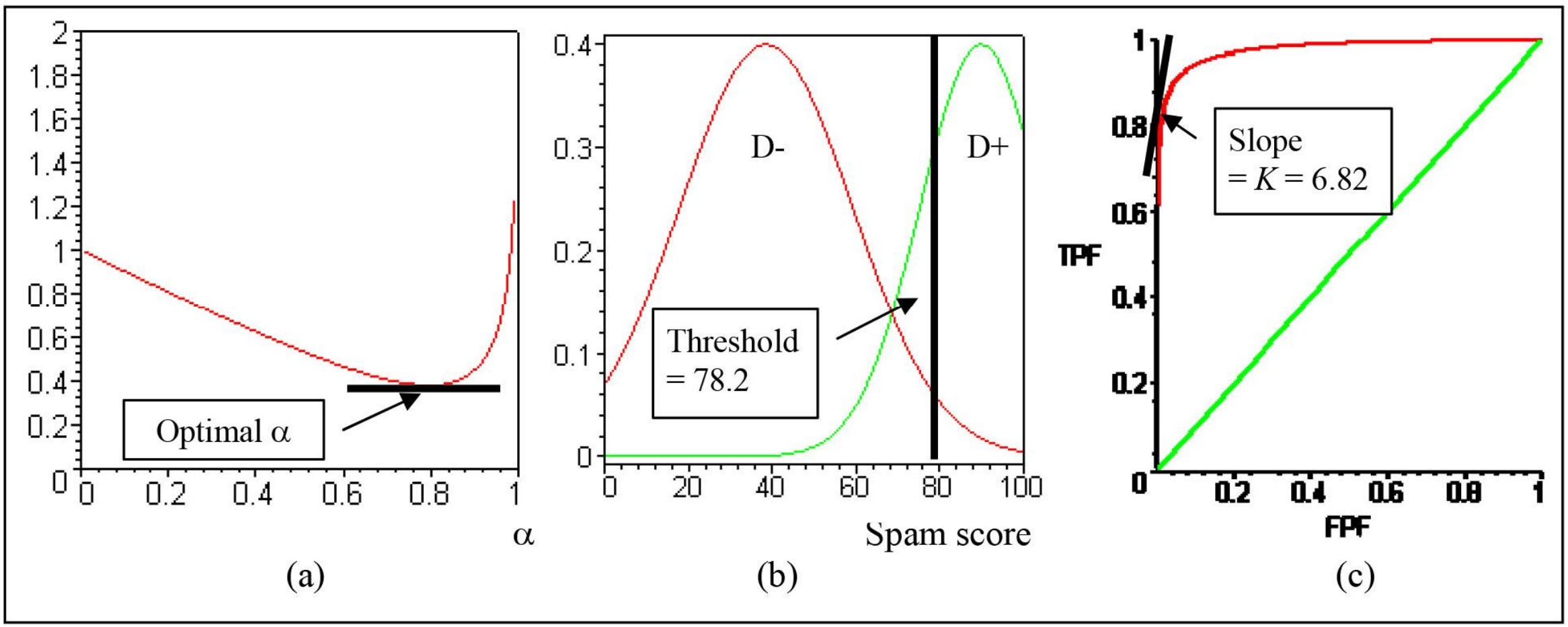
The optimal solution is found from Lemma 3: α* = Φ(AB + sqrt(A2 - 2(1 - B2) ln(BK))) / (1 - B2) = 79.7%. Since K is moderate - in other words, it is greater than 1 and less than 100 (for any B value) - we can find the unique optimal filtration level. The corresponding X* is Φ^-1(α*) = 0.83 and β* is Φ(A + BX) = 2.85%. From Φ((SS_i - μ_D+) / σ_D+) = α_i, or (SS_i) = μ_D+ - Φ^-1(α_i)σ_D+ for i=1 and 2, we compute (μ_D+ - σ_D+) = (89.8, 14.6). Then, the optimal threshold is x* = μ_D+ - σ_D+ Φ^-1(α*) = 78.2 from equation (1). The graph for two distributions with a spam score looks like Figure 9 (b). This α* can be computed from the ROC curve, where the slope is K. This is depicted in Figure 9 (c). However, the calculation of optimal value from the ROC curve is not as easy as from the original distributions. Lemma 4 identifies the direction of α* when other parameters change: This change is summarized in Table 2.
Table 2 Sensitivity analysis of the optimal solution with parameter changes
| Variables | New α* | Direction | Remarks |
|---|---|---|---|
| Base Model (A = -2.49, B = 0.71 and K = 6.12) | 0.797 | ||
| A = -3.00 (direction ↓) | 0.893 (↑) | $\frac{\partial \alpha^*}{\partial A} < 0$ | Decreasing A means increasing in the distance between the D+ and D- distributions. |
| B = 1.2 (↑) | 0.649 (↓) | $\frac{\partial \alpha^*}{\partial B} < 0$ for K < 71.2 | $\frac{\partial \alpha^*}{\partial B}$ > 0 for K > 71.2 where α* < 0.5 (i.e., for K < 71.2 very low filtration level). |
| K = 30 (↑) | 0.511 (↓) | $\frac{\partial \alpha^*}{\partial K} < 0$ | Since CFP becomes high, the solution reduces the FPF, resulting in lower α*. |
When we considered the double-threshold filtration system, we collected data on $C_{FP_i}$ and $C_{FN_i}$ for $i=1$ and 2. Note that this doesn’t change the distribution data for $D^+$ and $D^-$. Let assume $C_{FP_1}=50$, $C_{FP_2}=2$, $C_{FN_1}=0.5$, and $C_{FN_2}=1$. From Lemma 5(b), it is better off to use the double threshold. From
with $C_{FP_3}=C_{FN_0}=0$, we have $K_1=11.74$ and $K_2=0.489$. Using the solution for each $\alpha_1$ in Lemma 3, we have $\alpha_1=0.698$ (and the corresponding threshold $M_1=82.2$) and $\alpha_2=0.969$ ($M_1=62.6$). This means that if a certain e-mail has a spam score of greater than 82.2, the filter screens it and put it into the spam box (or does not deliver it); if an e-mail has a spam score between 62.6 and 82.2, the filter permits the message to be delivered with a warning in the subject line; if the e-mail has a spam score of 62.6 or less, the filter delivers it without any modification. Note that because of $K_1 > K_2$, it is better off to use the double-threshold system.
VI. Implications, Limitations, and Future Research
We have described the formulation of the total perceived cost of recovering FP and deleting FN to identify an optimal spam filtration level. Our analysis from the normal distribution shows that the optimal level depends on three parameters: A (the difference in mean values from two distributions - D+ and D-), B (the ratio of spread or standard deviation between two distributions), and K (the relative cost between recovering FP and deleting FN). Using these three variables, we discovered the optimal solution in the closed form. As the spam becomes more intelligent, A decreases and B increases, which results in less usage of anti-spam filters. The higher K is, the less we use anti-spam filters. We compared the new computing procedure with a ROC-based model. Parameters A and B can be obtained using only the results from two points of a filter performance test, without the need to construct the full ROC curve. Furthermore, we extended the new computing procedure to the multiple-threshold case and the non-normal distributions, even though some spam filtration systems normalize the raw spam scores (such as of Microsoft Exchange 2003).
The key steps to ensuring the analytical solution are: (a) demonstrating how to find two distributions with experimental values; (b) showing the shape of the curve for total cost; and (c) finding the optimal solution. Because three parameters are sufficient for finding the optimal filtration level, this result is easy to implement for most adaptive filters. Users’ perceived value for $\frac{C_{FP}}{C_{FN}}$ (or $\frac{C_{FP_i}-C_{FP_{i+1}}}{C_{FN_i}-C_{FN_{i-1}}}$ in general), the market (or an organization’s actual) data of distribution and rate of spam determine an optimal cutoff point for a given filter.
6.1 Implications
These results have several implications for managers. First, the model suggests a systematic method managers can use to determine an optimal filtration level for a firm. To our best knowledge, there have been no systematic ways for managers to determine a filtration level. Anecdotal evidence suggests that firms often simply use the default filtration level provided by vendors. We recommend that in deciding on an optimal filtration level, managers consider users’ total perceived costs of using an anti-spam filter. Second, given that FN and FP are identified as important factors influencing a firm's total perceived cost of an anti-spam filter, it is recommended that managers adopt the frequency of FN and FP as a main performance measure of an anti-spam filter. By monitoring the trend of the frequency of FN and FP, managers can assess how effectively an anti-spam filter serves users in an organization.
The most significant contribution of this study is to propose a practical model for determining the optimal spam-filtration level. Although previous research on the ROC curve implies a general idea about the relationship of FP and FN and about how to optimize, it has not been feasible for managers to actually apply the ROC-based method to real decision making because it was time consuming and difficult to determine an accurate optimal level as it needs tedious manual interventions: a) draw the ROC curve, b) calculate the optimal slope, and c) manually identify the optimal threshold point by finding the tangent of ROC curve. As a result, it was almost impossible to computerize management decisions on the optimal filtration level. Our new model overcomes these weaknesses of the ROC curve by using direct computations, opening an avenue for managers to automate decision making on the optimal filtration level.
The most important contribution of this study comes from wide applicability of this new model in many different domains. Our proposed model is applicable to numerous areas in which the ROC curve is typically employed, such as medical tests, speech recognition, and credit application evaluation (Krzanowski & Hand, 2009). In general, our model is applicable in cases where there are two groups that can be measured with a one-dimensional index. In addition to the areas in which the ROC curve is used, other potential applications are custom inspection for smuggled goods, security levels in airports, acceptance sampling in quality control, and so on. Although the parameters might be unique for a given environment, our research could be applied either as a general basis for reducing the harmful effects of FP and FN together or as a guideline to help managers identify future information requirements necessary in making an optimal decision.
6.2 Limitations and Future Research Topics
Although this paper shows the optimal filtration level for a given anti-spam filter, its findings should be interpreted within the context of several limitations of the research. First, the spam rate is currently about 46% of all e-mails, but this rate is not always applicable to a specific firm. As the spam summit described, e-mail addresses published in public websites receive more spam, because the spam mailers often use e-mail addresses harvested from public websites (FTC, 2007). Thus, it is recommended that anti-spam filters first block the blacklist and use content-based filtering triggered by certain words. After applying these methods, firms then can decide the spam rate for themselves. Our double-threshold filtration is more practical in this methodology. Second, it should be noted that parameters A and B must be reassessed when environmental conditions change. This implies that a few manual steps remain necessary in the proposed approach. Nevertheless, a key advantage of the proposed method is that, once the parameters are specified by the user, the optimal filtration level can be determined automatically, whereas ROC-based methods require a manual search for the optimal point. This feature could be seamlessly integrated into spam filter software. Third, users’ behavioral factors within the organization (e.g., how frequently they check the spam folder and whether they ignore warning messages) may significantly influence the perceived costs of false positives (FP) and false negatives (FN). The proposed model does not account for such individual-level behaviors; instead, it incorporates aggregate costs at the organizational level. Fourth, $\delta C_{FN}$ is not included in deriving the first-order condition, as a linear cost function is assumed. Extending the model to incorporate more general cost functions remains an important direction for future research. Fifth, the practical implementation of the proposed dual-threshold system and its associated costs were not examined in this study and remain subjects for future research. Lastly, determining user-perceived costs effectively and in a timely manner within an organization is an important issue that was not addressed in this study. It remains a topic for future research. The user perceived costs should be reassessed regularly by receiving user feedback. The more rigorous filtration users prefer, the lower K (or $\frac{CFP}{CFN}$) the filter applies for the new computation of $\alpha^*$, or vice versa. This procedure can be automatically implemented by receiving users feedback.
APPENDIX
(Proof of Observation 1)
From equation (7), $\beta = \Phi(A + BX)$ where $X = \Phi^{-1}(\alpha)$. Thus, we have $A + B\Phi^{-1}(\alpha) = \Phi^{-1}(\beta)$. For $\Phi^{-1}(\alpha_1) \neq \Phi^{-1}(\alpha_2)$, the determinant of linear equations of $A + B\Phi^{-1}(\alpha_1) = \Phi^{-1}(\beta_1)$ and $A + B\Phi^{-1}(\alpha_2) = \Phi^{-1}(\beta_2)$ should not be zero, and thus there exists a unique solution for A and B.
(Proof of Lemma 2)
(a) If B = 1, $C''(\alpha) = \frac{K(-A)\phi(A+X)}{\phi(X)^2} > 0$ for any $\alpha$ because A < 0. Thus, $C''(\alpha) > 0$ for all $\alpha$.
(b) If B ≠ 1, we have a unique $X_1 = AB/(1-B^2)$ satisfying $C''(\alpha) = 0$. Thus, the inflection point $\alpha$ is $\Phi\left(\frac{AB}{1-B^2}\right)$. As $\alpha$ increases, X increases and (11) changes from negative to positive for B < 1. Thus, C($\alpha$) moves from concave to convex.
(c) For B > 1, since X decreases in $\alpha$, C($\alpha$) moves from convex to concave.
(Proof of Lemma 3)
The optimal solution satisfies the FOC, in the convex region. From $\phi(x) = \frac{1}{\sqrt{2\pi}} \exp\left(-\frac{x^2}{2}\right)$, $\frac{\phi(X)}{\phi(A+BX)} = \frac{\exp(-X^2/2)}{\exp(-(A+BX)^2/2)} = \exp\left(-\frac{(1-B^2)X^2 - 2ABX - A^2}{2}\right)$. Thus, the FOC from (10) is simplified to $(1 - B^2)X^2 - 2ABX - A^2 + 2 \ln(BK) = 0$. (14) Solving this equation, we can obtain the optimal X* and then calculate $\alpha^* = \Phi(X^*)$.
(a) If B = 1, $X^* = \frac{-2\ln(BK)-A^2}{2AB} = \frac{2\ln(K)-A^2}{2A}$ and thus $\alpha^* = \Phi\left(\frac{2\ln(K)-A^2}{2A}\right)$.
(b) If B ≠ 1, the determinant of quadratic (14), D, is $D = (AB)^2 - 1(1 - B^2)(-A + 2 \ln(BK)) = A^2 - 2(1 - B^2) \ln(BK)$ (15) If D < 0, then there is no real solution for X, and the LHS (left-hand-side) of (14) has the same sign as 1 - B2 for all X. This results in C($\alpha$) decreasing in the whole region for 1 - B2 < 0 or B > 1, and the optimal $\alpha^*$ should be 1. The reverse is true for B < 1, and optimal $\alpha^*$ should be 0.
(c) If B ≠ 1 and D > 0, there exist two solutions satisfying (14): $X_1 = \frac{AB-\sqrt{D}}{1-B^2}$ and $X_2 = \frac{AB+\sqrt{D}}{1-B^2}$. The optimal solution to minimize the C($\alpha$) exists in the convex region, and AB(1 - B2) is an inflection point in X. From Lemma 2, if B > 1, C($\alpha$) changes from convex to concave in $\alpha$, and also in X. Thus, the optimal solution to minimize C($\alpha$) is a smaller one from X1 and X2. Since 1 - B2 < 0, X2 is smaller. In the same stream, if B < 1 where C($\alpha$) changes from concave to convex in X, the optimal solution is X2. Although there is a unique local optimal $\alpha^*$ in the convex region, if D is not large enough, we may still find the solution in the boundary, i.e., $\alpha = 0$ for B < 1 or $\alpha = 1$ for B > 1, similar to part (b). From (9), $C(\alpha = 0) \lim_{x \to \infty} [1 - \Phi(X) + K \cdot \Phi(A + BX)] = 1$ and $C(\alpha = 1) = \lim_{x \to \infty} [1 - \Phi(X) + K \cdot \Phi(A + BX)] = K \cdot C(\alpha^*)$ should be compared with the boundary value C(0) = 1 or C(1) = K.
(Proof of Lemma 4)
(a) Since $\frac{\partial \alpha^*}{\partial A} = \phi(X^*) \cdot \frac{\partial X^*}{\partial A}$, the sign of $\frac{\partial \alpha^*}{\partial A}$ is the same as that of $\frac{\partial X^*}{\partial A}$. From $X^* = \frac{AB + \sqrt{D}}{1 - B^2}$ and (15), For $K > \exp(-\frac{A^2}{2B^2})$, $\frac{\partial X^*}{\partial A} < 0$. Since $\exp(-\frac{A^2}{2B^2})$ is always less than 1 for B > 1 and for A > -0.6 (very low discriminability) and B < 1, we can conclude $\frac{\partial \alpha^*}{\partial A} < 0$ for K > 1 in general.
(b) From $\frac{A^2 - D}{2(1 - B^2)} = \ln(BK)$, $\frac{\partial D}{\partial B} = 4B \ln(BK) - \frac{2(1 - B^2)}{B} = \frac{2(A^2 - D)}{B} - \frac{2(1 - B^2)}{B}$. Similarly to part (a), The solutions of D satisfying are $\frac{-A(1 + B^2) \pm (1 - B^2)\sqrt{A^2 + 4}}{2B}$, say D1 and D2. From $D = A^2 - 2(1 - B^2) \ln(BK)$, the two K's can be calculated from D1 and D2. The bigger K value, K2, comes from From $\ln(BK_2)$, $K_2 = \frac{1}{B} \exp(-\frac{A(1 + B^2)\sqrt{A^2 + 4} + (A^2 + 2)(1 - B^2)}{4B^2})$. In the same way, K1 = $\frac{1}{B} \exp(-\frac{A(1 + B^2)\sqrt{A^2 + 4} + (A^2 + 2)(1 - B^2)}{4B^2})$ from D1 is negative for K between K1 and K2, and positive otherwise. Note that K1 (that is, lower bound of K) is small enough to be ignored as shown in Figure 10(b).
(c) $\frac{\partial X^*}{\partial K} = \frac{1}{1 - B^2} (\frac{1}{2\sqrt{D}} \cdot \frac{\partial D}{\partial K}) = \frac{1}{2(1 - B^2)\sqrt{D}} (-\frac{2(1 - B^2)}{K}) = -\frac{1}{K\sqrt{D}} < 0$
저자 약력
∙ Richard K. Cho is an Associate Professor in the OIM area of the Faculty of Business at University of New Brunswick (UNB) in Saint John. He holds degrees from Seoul National University (B.Sc.), KAIST (M.Sc.), and the University of Waterloo (Ph.D.). Before joining UNB, he taught at Wilfrid Laurier University and Purdue University’s Krannert School of Management. His research focuses on supply chain management, logistics, inventory, and game theory. He is a recipient of two SSHRC grants, and his work has appeared in leading journals such as Operations Research, Manufacturing & Service Operations Management, International Journal of Production Economics, IIE Transactions, and the European Journal of Operational Research.
∙ Dr. Dongmin Kim is a Professor of MIS at the University of New Brunswick in Saint John. He earned his Ph.D. from the University of British Columbia, an MBA in MIS, and a B.A. in Economics from Yonsei University. Before joining academia, he had worked for 17 years at IBM Korea. His research focuses on online trust, user interfaces in e-commerce, and business analytics, including no-code and low-code tools. He has published in two Financial Times 50 journals—Information Systems Research and Journal of MIS—and is a recipient of two Social Sciences and Humanities Research Council (SSHRC) grants.
∙ Dr. Jong-Kyou Kim is an Assistant Professor in the Department of Computer Science at the University of New Brunswick, Saint John. He earned his Ph.D., M.Sc., and B.C.S. from Korea Advanced Institute of Science and Technology. Prior to his academic role, he spent 15 years working with Technology Companies – including Mirae Corporation, TmaxSoft, and kt innotz – focusing on leveraging data analytics and machine learning for operational improvements. While in industry, he also instructed at NHN Next, Kookmin University, and Korea University in Korea. Dr. Kim’s research interests center on the application of advanced analytics, particularly in Artificial Intelligence and big data processing, to optimize complex systems and informed decision-making. His recent publications have appeared in SCI journals and conferences. He is a recipient of an NBIF grant (New Brunswick Innovation Fund).