.jpeg)
Your Movement in a City Reveals Your Credit: Credit Default Prediction Based on Geolocation Information
1 Shanghai Jiao Tong University
2 Yonsei University
DOI: https://doi.org/10.17287/kmr.2026.55.1.285
Abstract
Do individuals at high risk of credit default frequent different locations within a city than those at low risk? Leveraging large-scale geolocation data, we propose that geosimilarity risk and geolocation network size serve as novel and informative classifiers for predicting individual credit default. We define two individuals as geosimilarity network (GSN) neighbors if they share at least one visited location during a given period. Using consumer location traces combined with loan repayment histories from a leading Fin Tech company, we find that the GSN neighbors of a defaulter are approximately three times more likely to default than the average borrower and about 4.5 times more likely to default than the GSN neighbors of a non-defaulter. Moreover, geosimilarity risk and geolocation network size significantly explain default outcomes after controlling for traditional factors such as demographics, financial capacity, and loan characteristics. Incorporating these geolocation-based measures into standard credit risk models improves predictive accuracy by approximately 9 percent. These findings highlight the value of spatial mobility data as a complementary source of information for credit risk assessment.
Ⅰ. Introduction
Lending and borrowing date back to 2000 B.C., when organized economic exchange first emerged (Thomas et al., 2017). At the core of these activities are creditworthiness and trust, which credit scoring seeks to quantify systematically (Hand and Jacka, 1998). As the credit industry has expanded, credit scoring has become a critical tool for banks and has been applied across domains such as marketing, engineering, manufacturing, healthcare, and medicine (Abdou and Pointon, 2011).
Despite its widespread use, much of the credit scoring literature has emphasized methodological refinements, particularly advanced statistical and machine learning techniques for distinguishing high- and low-risk borrowers (Abdou and Pointon, 2011). By contrast, limited progress has been made in identifying new classifiers for credit risk assessment. Existing models primarily rely on demographic information, financial records, and loan-specific characteristics embedded in credit bureau reports. However, global coverage of such data remains limited. Only 13% of adults have repayment or debt information recorded in public credit registries, and just 31% are covered by private credit bureaus (World Bank, 2017). In many developing countries, disaggregated demographic data are also unavailable (Blumenstock et al., 2015), making the establishment of effective credit systems a persistent global challenge.
By contrast, mobility data are abundant. Advances in digital technologies, particularly the diffusion of the Internet and mobile phones, have resulted in the pervasive presence of location-based information (de Montjoye et al., 2013). Approximately 5.2 billion individuals worldwide use Internet-enabled mobile phones (Mundial, 2016), which has resulted in large-scale location-visitation data worldwide.
In this study, we examine whether geo-location data can serve as a proxy for credit risk. Our approach is motivated by prior research showing that location visitation patterns provide informative signals of similarity among individuals (Provost et al., 2015). Individuals who frequent the same places often share similar interests, social backgrounds, and consumption habits. For example, visits to luxury department stores or casinos may convey information about wealth or lifestyle, whereas visits to neighborhood coffee shops may signal housing affordability. Prior studies further show that geographical co-occurrence predicts friendships (Crandall et al., 2010) and mobile app adoption (Pan et al., 2011). Building on this literature, we propose that geosimilar individuals, defined as those who visit at least one common location within a given period, are likely to exhibit similar levels of credit risk. Importantly, geosimilarity does not require co-presence or interpersonal ties, as individuals may visit the same location at different times.
Beyond similarity, social stigma costs may also influence borrowing behavior. Borrowers experiencing financial distress often seek to conceal their loan-related activities, particularly when they face an elevated risk of bankruptcy. Because of stigma associated with visible financial need (Thorne and Anderson, 2006), high-risk borrowers may prefer private settings, such as their homes, for loan applications or credit checks, whereas low-risk borrowers may be more comfortable accessing lender websites from public locations. As a result, the number and diversity of public locations from which borrowers interact with a lender may serve as informative indicators of credit risk.
To evaluate these ideas, we leverage a large-scale dataset from a leading Fin Tech company in Hong Kong that combines consumer location traces with loan repayment histories. Following the Geo-Similarity Network framework proposed by Provost et al. (2015), we construct four geolocation-based variables, including three measures of geosimilarity credit risk and one measure of geolocation network size that captures potential stigma-related effects. We empirically assess their predictive power alongside traditional credit risk variables.
Our findings indicate that the GSN neighbors of a defaulter are approximately three times more likely to default than the average borrower and 4.5 times more likely to default than the GSN neighbors of a non-defaulter. These results suggest that high- and low-risk borrowers tend to cluster spatially within cities. We also find evidence consistent with stigma costs, as borrowers with larger geolocation networks are less likely to default. Overall, geosimilarity risk and geolocation network size significantly explain credit default after controlling for conventional demographic, financial, and loan-level predictors. Incorporating geolocation features into standard models improves prediction accuracy by approximately 9 percent. These findings indicate that geolocation data provide meaningful cues about borrower creditworthiness, particularly in contexts where conventional financial and demographic information is unavailable.
Ⅱ. Related Literature
This study builds on and contributes to two streams of research. The first stream focuses on the development of credit default models, which rely on demographic, financial, and loan-specific variables and employ increasingly sophisticated statistical and machine learning techniques. The second stream is rooted in location analytics, which seeks to generate managerial insights from consumer geolocation data and their behaviors across locations.
2.1 Credit Default Models
Although lending and borrowing have existed for more than 4,000 years, systematic credit scoring that assigns numerical or alphabetical scores to indicate default risk was not empirically studied until modern financial institutions and credit bureaus began recording individual-level credit activities (Abdou and Pointon, 2011). Empirical studies on individual credit models remain limited, however, because financial activities and credit information are among the most sensitive data to obtain and analyze (Phelps et al., 2000).
Table 1 Types of Predictors in Credit Default Models
| Predictor Type | Examples | Representative Studies |
|---|---|---|
| Demographic Characteristics | age, gender, marital status, education, occupation | Lawrence et al. (1992); Stepanova and Thomas (2002); Jiang et al. (2018); Steenackers and Goovaerts (1989) |
| Financial Ability Measures | credit scores, monthly income, bank accounts, asset ownership, mortgage information | Barth et al. (1983); Steenackers and Goovaerts (1989); Lawrence et al. (1992); Stepanova and Thomas (2002); Šušteršič et al. (2009) |
| Loan-Specific Variables | loan amount, tenor, interest rate | Barth et al. (1983); Lawrence et al. (1992); Stepanova and Thomas (2002); Jiang et al. (2018) |
| P2P Platform and Social Network Variables | friendship networks, social ties, relational herding, textual soft information, message framing | Lin et al. (2013); Liu et al. (2015); Wei et al. (2016); Jiang et al. (2018); Huang et al. (2021) |
| Geolocation Measures | geosimilarity risk, geolocation network size | This study |
More recently, with the rise of the Fin Tech industry, attention has shifted toward peer-to-peer (P2P) lending platforms, where individual lenders and borrowers are matched (Bao et al., 2024; Lin et al., 2013; Liu et al., 2015; Jiang et al., 2018; Huang et al., 2021; Pena and Breidbach, 2021), and toward the role of social networks in improving loan performance (Lin et al., 2013; Liu et al., 2015; Wei et al., 2016).
Across these contexts, credit default models have primarily relied on three core categories of predictors, which capture demographic characteristics, financial ability measures, and loan-specific variables. These predictors constitute the conventional information set used in most traditional credit risk models.
Demographic characteristics such as age, gender, marital status, education, and occupation capture stable individual attributes that may correlate with financial responsibility and repayment behavior (Lawrence et al., 1992; Stepanova and Thomas, 2002). Financial ability measures including credit scores, income, asset ownership, and debt levels directly assess the borrower's capacity to service debt obligations (Barth et al., 1983; Šušteršič et al., 2009). Loan-specific variables such as principal amount, tenor, and interest rate reflect the risk profile of the particular transaction and the lender's risk assessment at origination (Jiang et al., 2018).
Our study extends this literature by introducing geolocation measures, including geosimilarity and geolocation network size, as a new category of predictors for individual credit default. Unlike the traditional predictor types, geolocation features capture behavioral patterns and social context derived from spatial mobility data. This represents a fundamental expansion of the information set available for credit risk assessment, particularly in settings where traditional financial and demographic data are sparse or unavailable.
2.2 Location Analytics and Spatial Economics
A second stream of related research is location analytics, which has gained traction in Information Systems and Marketing due to the proliferation of mobile devices and the resulting availability of consumer geolocation data (e.g., Fang et al., 2015; Narang and Luco, 2025). However, the informational value of location data extends beyond marketing applications and is grounded in fundamental principles from multiple disciplines including urban economics, economic geography, and social network theory.
The theoretical foundation for using geolocation data as a predictor of credit risk rests on two well-established mechanisms, homophily and spatial clustering. Homophily, defined as the tendency for similarity to foster connection, is one of the most robust findings in social network research (Mc Pherson et al., 2001). This principle suggests that individuals tend to associate with others who are similar to themselves in terms of socio-demographic characteristics, attitudes, behaviors, and life circumstances. Importantly, homophily manifests not only in social ties but also in spatial co-location patterns. People with similar backgrounds, preferences, and behavioral tendencies are more likely to frequent the same types of places, even without direct social interaction.
Economic geography and urban economics provide complementary perspectives on why individuals with similar economic characteristics cluster spatially. Florida (2004) suggests that individuals with similar occupational profiles and income levels tend to concentrate in specific neighborhoods and patronize similar establishments. Glaeser et al. (2001) highlight that urban spatial arrangements reflect and reinforce consumption patterns and economic opportunities, creating localized agglomerations of similar consumers. Consistent with this view, prior research shows that location-specific contexts shape consumer choices by interacting with economic constraints and situational factors (Molitor et al., 2016).
In the context of credit risk, these mechanisms imply that individuals who visit the same locations tend to share similar financial circumstances and behaviors. Visits to luxury department stores or casinos may signal wealth or risk-taking tendencies, whereas visits to discount retailers or community welfare centers may indicate financial constraints. Geosimilarity, defined as sharing visited locations, does not require physical co-presence or direct social interaction, as individuals may visit the same locations at different times. Shared location choices nonetheless reveal similarities in socioeconomic status, lifestyle, and potentially creditworthiness.
Beyond similarity-based clustering, social stigma provides a second theoretical mechanism linking geolocation patterns to credit risk. Social stigma theory, rooted in sociology and social psychology (Goffman, 1963; Link and Phelan, 2001), posits that individuals seek to manage potentially discrediting information about themselves to avoid social devaluation. Financial distress carries significant social stigma in many cultures, leading individuals to engage in impression management strategies to conceal their economic vulnerability (Thorne and Anderson, 2006).
In borrowing behavior, stigma costs are reflected in spatial choices. Borrowers experiencing financial distress may prefer to conduct loan-related activities in private settings, such as their homes, in order to avoid social observation and judgment. This privacy-seeking behavior reflects concerns about reputational damage and social embarrassment associated with visible financial need. By contrast, borrowers with greater financial confidence may access lending platforms from a wider range of public locations, including offices, cafes, and libraries.
Accordingly, the size and diversity of a borrower’s geolocation network may serve as a behavioral signal of financial confidence or distress. Consistent access from only one or two private locations may indicate stigma-related concealment, whereas access from a broader set of locations may signal lower perceived stigma and reduced financial vulnerability.
Ⅲ. Geolocation Network and Geosimilarity
We adopt the GSN design proposed by Provost et al. (2015). Figure 1 illustrates the procedure for identifying geosimilar individuals.
We begin by constructing a GSN for each person (here, person X) based on all IP addresses observed for that individual during a given period. Any other individual who has visited at least one of these IP addresses during the same period is considered a neighbor of person X. For example, persons A, B, C, and D are identified as neighbors of person X. The location profile of each individual is represented as a vector, where element i denotes whether or not that person has visited location IPi. The five individuals in Figure 1 can be expressed as follows:
$\vec{x}_X = [1, 1, 1, 1], \vec{x}_A = [1, 1, 0, 0], \vec{x}_B = [0, 1, 1, 0],$ $\vec{x}_C = [0, 0, 1, 0], \vec{x}_D = [0, 0, 0, 1]$
We define three measures of geosimilarity. The first measure (M1) assigns a similarity of 1 if two individuals share at least one location and 0 otherwise. In this case, persons A, B, C, and D are equally geosimilar to person X. The second measure (M2) weights similarity by the number of shared locations, such that persons A and B are more geosimilar to person X than persons C and D, since the former share two locations while the latter share only one. The third measure (M3) further adjusts for location popularity. For instance, suppose IP1 corresponds to Times Square in New York City, whereas IP3 represents a local coffee bar near person X's residence. Although both persons A and B share two locations with X, person B may be regarded as more geosimilar because IP3 is less frequently visited. To capture this, we introduce a popularity discount factor, $w_i$, defined as the logarithm of the total population n divided by the number of individuals who visited location IPi. This is analogous to the inverse document frequency weighting commonly used in text mining (Hotho et al., 2005). For example, if $n = 10$ and the number of visitors to IP1, IP2, IP3, and IP4 are 4, 3, 2, and 1 respectively, the discount vector is:
$\vec{w} = [0.4, 0.5, 0.7, 1]$
We hypothesize that the default risk of an individual is related to the default risk of their GSN neighbors. The GSN default risk is defined as the average loan default rate of neighbors, weighted by geosimilarity:
where $D_j$ equals 1 if GSN neighbor $j$ defaults, and 0 otherwise. Table 2
Table 2 Geosimilarity Measures and GSN Default Risk of Person X when Person B Defaults
| Geosimilarity | $S_{X,A}$ | $S_{X,B}$ | $S_{X,C}$ | $S_{X,D}$ | GSN default risk | |
|---|---|---|---|---|---|---|
| $M1$ | $S_{i,j}(\vec{x}_i, \vec{x}_j) = \min(\vec{x}_i \cdot \vec{x}_j, 1)$ | 1 | 1 | 1 | 1 | 0.250 |
| $M2$ | $S_{i,j}(\vec{x}_i, \vec{x}_j) = \vec{x}_i \cdot \vec{x}_j$ | 2 | 2 | 1 | 1 | 0.333 |
| $M3$ | $S_{i,j}(\vec{x}_i, \vec{x}_j) = (\vec{w} \circ \vec{x}_i) \cdot \vec{x}_j$ | 0.9 | 1.2 | 0.7 | 1 | 0.315 |
Note: For illustration, the GSN default risk in column 6 considers the default of persons A, B, C, D only.
We also posit that social stigma costs may be reflected in borrowers' geolocation network size, measured by the number of unique IP addresses from which a borrower accesses the Fin Tech platform. A greater number of unique access points indicates that the borrower interacted with the platform from multiple locations, which may signal lower stigma-related concerns and, in turn, lower default risk.
When working with mobility data, privacy concerns are paramount. To address these concerns, we adopt a doubly anonymized design, in which both device identifiers and location identifiers are replaced with random numbers. Under this approach, the analyst does not know the actual locations visited by applicants but only whether they visited the same location and how many unique locations were recorded. This privacy-preserving mechanism ensures that the method is both analytically useful and practically feasible, given the sensitive nature of geolocation data.
Ⅳ. Empirical Analysis
4.1 Data and Variable Selection
We obtained a large-scale dataset from a leading Fin Tech platform in Hong Kong whose primary business is consumer lending. Unlike traditional banks, the platform allows applicants to request loans online without submitting extensive documentation. The dataset includes conventional credit scoring factors such as demographics, financial information (e.g., credit grades from the Hong Kong credit bureau, income, and debt), loan characteristics, and the IP addresses through which customers accessed the platform. In our context, therefore, location information represents the online footprints of borrowers.
Between June 2013 and April 2017, 48,712 unique applicants submitted 82,066 loan requests. The company approved 18,763 of these applications. Among the approved borrowers, 10,390 had at least one GSN neighbor, while 2,056 had no neighbors, meaning they accessed the platform only from a private IP address (e.g., at home).
Applicants provide both self-reported and observational data. During the application process, they fill out an online form requiring demographic and financial details, including gender, age, occupation, monthly income, current debt, and proposed loan amount and tenor. Submission of a Hong Kong ID number is mandatory, allowing the platform to retrieve official credit reports from the Hong Kong credit bureau. If self-reported information substantially differs from official records, the application is rejected. Following prior literature, our models include the proposed loan amount, proposed tenor, two-year interest rate, monthly income, gender, and age (variables: Original_amount, Original_tenor, Two-year_interest_rate, Monthly_income, Female, Age).
The platform’s credit grade system, based on bureau reports, ranges from Grade 1 (lowest risk) to Grade 11 (highest risk). We incorporate this measure by including ten dummy variables (GradeX, where X = 1 to 10). We also include the debt-to-income ratio, widely used in lending to evaluate repayment capacity.
In addition to financial information, our dataset contains detailed IP address histories for each applicant. On average, borrowers used eight distinct IP addresses to log into the platform. We treat each unique IP address as a unique location. Although this dataset does not capture full mobility traces, prior research shows that as few as four distinct locations are sufficient to identify 95% of individuals (de Montjoye et al., 2013). Importantly, location choices carry behavioral meaning. Borrowers may avoid logging in from public spaces due to privacy concerns, particularly when experiencing financial distress (Thorne and Anderson, 2006; Chen and Guestrin, 2016). To capture this phenomenon, we define GSN size as the number of unique IP addresses associated with a borrower, which may reflect stigma-related constraints.
A potential limitation in mobility datasets is that individuals using multiple Internet-enabled devices (e.g., smartphones, PCs) may be mistakenly treated as distinct users. Our dataset avoids this problem, as the platform assigns a unique identifier to each individual, regardless of device, thereby eliminating double-counting.
Finally, the platform tracks loan performance monthly. Once approved, a loan becomes “active.” Loans are classified as “default” if the borrower fails to make repayments for four consecutive months, and as “settled” if repaid in full at maturity. For empirical analysis, we exclude all currently active loans, focusing only on loans with observed outcomes (defaulted or settled).
4.2 Comparison of Loans by Loan Status
Table 3 Summary Statistics
| Panel A: | Defaulted Loans (nDL = 574) | ||||
|---|---|---|---|---|---|
| Mean | Std. | Median | Min | Max | |
| GSN size | 6.0 | 6.2 | 4.0 | 1.0 | 54.0 |
| Original_tenor (days) | 834.6 | 429.9 | 720.0 | 120.0 | 1800.0 |
| Original_amount (HKD) | 80780.4 | 83161.8 | 50000.0 | 3000.0 | 600000.0 |
| Monthly_income (HKD) | 19166.0 | 11892.7 | 16000.0 | 7200.0 | 157848.0 |
| Debt-to-income ratio | 10.8 | 7.0 | 9.7 | 0.4 | 35.0 |
| Two-year_interest_rate | 51.2 | 149.7 | 9.0 | 2.0 | 2177.0 |
| Age | 44.9 | 13.4 | 48.8 | 0.0 | 59.8 |
| Gender (M=1, F=2) | 1.2 | 0.4 | 1.0 | 1.0 | 2.0 |
| Panel B: | Settled Loans (nNDL = 8091) | ||||
| GSN size | 11.4 | 9.8 | 9.0 | 1.0 | 97.0 |
| Original_tenor (days) | 747.4 | 447.9 | 720.0 | 14.0 | 1800.0 |
| Original_amount (HKD) | 74375.1 | 83882.2 | 50000.0 | 3000.0 | 600000.0 |
| Monthly_income (HKD) | 21488.9 | 21342.3 | 17025.5 | 0.0 | 1338836.0 |
| Debt-to-income ratio | 11.1 | 7.1 | 9.8 | 0.1 | 107.3 |
| Two-year_interest_rate | 165.9 | 198.1 | 102.0 | 1.0 | 2088.0 |
| Age | 36.3 | 16.7 | 38.7 | 0.0 | 60.0 |
| Gender (M=1, F=2) | 1.2 | 0.4 | 1.0 | 1.0 | 2.0 |
| Panel C: | All Disbursed Loans (nADL = 8665) | ||||
| GSN size | 11.0 | 9.7 | 8.0 | 1.0 | 97.0 |
| Original_tenor (days) | 753.2 | 447.3 | 720.0 | 14.0 | 1800.0 |
| Original_amount (HKD) | 74798.9 | 83845.0 | 50000.0 | 3000.0 | 600000.0 |
| Monthly_income (HKD) | 21335.1 | 20857.0 | 17000.0 | 0.0 | 1338836.0 |
| Debt-to-income ratio | 11.1 | 7.1 | 9.8 | 0.1 | 107.3 |
| Two-year_interest_rate | 158.3 | 197.4 | 92.0 | 1.0 | 2177.0 |
| Age | 36.8 | 16.6 | 39.8 | 0.0 | 60.0 |
| Gender (M=1, F=2) | 1.2 | 0.4 | 1.0 | 1.0 | 2.0 |
| Panel D: | Accepted Loans (nAL = 17638) | ||||
| GSN size | 9.0 | 8.5 | 6.0 | 1.0 | 97.0 |
| Original_tenor (days) | 858.3 | 476.6 | 720.0 | 14.0 | 1800.0 |
| Original_amount (HKD) | 87891.0 | 99872.4 | 50000.0 | 3000.0 | 600000.0 |
| Monthly_income (HKD) | 22147.2 | 22458.8 | 17254.0 | 0.0 | 1338836.0 |
| Debt-to-income ratio | 12.1 | 7.8 | 10.7 | 0.1 | 107.3 |
| Two-year_interest_rate | 144.1 | 178.7 | 87.0 | 1.0 | 2177.0 |
| Gender (M=1, F=2) | 1.2 | 0.4 | 1.0 | 1.0 | 2.0 |
| Panel E: | Non-accepted Loans (nNAL = 44227) | ||||
| GSN size | 5.3 | 7.1 | 3.0 | 1.0 | 93.0 |
| Original_tenor (days) | 866.5 | 500.4 | 720.0 | 14.0 | 1800.0 |
| Original_amount (HKD) | 88860.6 | 106990.4 | 50000.0 | 3000.0 | 600000.0 |
| Monthly_income (HKD) | 59893.4 | 7611335.0 | 16000.0 | 0.0 | 1597016000.0 |
| Debt-to-income ratio | 15.4 | 13.4 | 12.5 | 0.0 | 429.4 |
| Two-year_interest_rate | 110.4 | 164.1 | 46.0 | 1.0 | 2177.0 |
| Gender (M=1, F=2) | 1.2 | 0.4 | 1.0 | 1.0 | 2.0 |
| Panel F: | All Loans (nAll = 61865) | ||||
| GSN size | 6.4 | 7.7 | 4.0 | 1.0 | 97.0 |
| Original_tenor (days) | 864.2 | 493.7 | 720.0 | 14.0 | 1800.0 |
| Original_amount (HKD) | 88583.8 | 105007.4 | 50000.0 | 3000.0 | 600000.0 |
| Monthly_income (HKD) | 49144.4 | 6437012.0 | 16590.0 | 0.0 | 1597016000.0 |
| Debt-to-income ratio | 14.4 | 12.1 | 11.8 | 0.0 | 429.4 |
| Two-year_interest_rate | 120.0 | 169.1 | 55.0 | 1.0 | 2177.0 |
| Gender (M=1, F=2) | 1.2 | 0.4 | 1.0 | 1.0 | 2.0 |
Table 4 Number of Applications by Credit Grade
| Credit grade | Application | Approved | Rejected | Defaulted | Settled |
|---|---|---|---|---|---|
| 1 | 208 | 59 | 149 | 0 | 62 |
| 2 | 545 | 212 | 333 | 1 | 213 |
| 3 | 1804 | 727 | 1077 | 3 | 740 |
| 4 | 1978 | 822 | 1156 | 6 | 838 |
| 5 | 2913 | 1190 | 1723 | 11 | 1219 |
| 6 | 7689 | 2915 | 4774 | 39 | 2946 |
| 7 | 7297 | 2462 | 4835 | 63 | 2451 |
| 8 | 15463 | 4753 | 10710 | 205 | 4631 |
| 9 | 12353 | 3124 | 9229 | 222 | 2954 |
| 10 | 5221 | 77 | 5144 | 20 | 57 |
| 11 | 2920 | 839 | 2081 | 48 | 798 |
Note: The total number of Defaulted and Settled is not equal to the number of Approved because the applicant has the right to decide whether to accept the approved loan.
4.3 Empirical Analysis
We begin by comparing GSN measures between defaulted and settled loans. Figure 2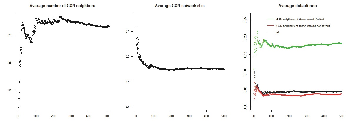
If geosimilarity indeed reflects credit default risk, then GSN default risk measures based on the three geosimilarity definitions (M1, M2, and M3, hereafter RM1, RM2, and RM3) should be significantly associated with loan default. Moreover, the informativeness of these measures should increase as more weight is assigned to highly geosimilar neighbors. Our baseline empirical tests evaluate both the statistical significance and the economic magnitude of these effects. This approach is consistent with prior studies that assess default prediction models based on their classification performance and discriminative power (Park and Ahn, 2014).
We estimate logit models, as the dependent variable is a binary indicator of loan default. A loan is classified as default when repayments are overdue by at least 120 days. We run three regressions, each including one of the standardized GSN default risk measures (RM1, RM2, and RM3). In addition, we incorporate GSN size to capture the effect of social stigma costs.
We start our analysis with the accepted loans of applicants with GSN neighbors. Our dependent variable is a dummy (Di) for each borrower i, which equals 1 if her loan defaults, and 0 otherwise. Our variables of interest are the three GSN default risks (GSN default riski) and GSN size (GSN sizei) for each borrower I:
The control variables, consistent with prior research and industry practice, include credit grade, monthly income, and debt-to-income ratio (all from the Hong Kong credit bureau). We further include loan-specific characteristics such as principal, tenor, and interest rate, as well as demographic variables (gender and age).
Table 5 Logistic Regression: All Disbursed Loans of Those Who Have GSN Neighbors
| (1) | (2) | (3) | (4) | |
|---|---|---|---|---|
| GSN RM1 | 0.171*** | |||
| (0.035) | ||||
| GSN RM2 | 0.177*** | |||
| (0.035) | ||||
| GSN RM3 | 0.179*** | |||
| (0.035) | ||||
| GSN_size | -0.136 | -0.136 | -0.136*** | |
| (0.011) | (0.011) | (0.011) | ||
| Grade10 | 1.522 | 1.030 | 1.028 | 1.026 |
| (0.332) | (0.361) | (0.361) | (0.361) | |
| Grade9 | 0.325* | 0.276 | 0.274 | 0.274 |
| (0.174) | (0.182) | (0.182) | (0.182) | |
| Grade8 | -0.084 | -0.263 | -0.264 | -0.265 |
| (0.180) | (0.187) | (0.187) | (0.187) | |
| Grade7 | -0.403 | -0.537 | -0.544 | -0.545* |
| (0.221) | (0.232) | (0.232) | (0.232) | |
| Grade6 | -0.783 | -1.009 | -1.012 | -1.013 |
| (0.253) | (0.267) | (0.267) | (0.267) | |
| Grade5 | -1.154 | -1.431 | -1.434 | -1.435 |
| (0.406) | (0.434) | (0.434) | (0.434) | |
| Grade4 | -1.123 | -1.387 | -1.391 | -1.392* |
| (0.499) | (0.506) | (0.506) | (0.506) | |
| Grade3 | -1.664 | -1.924 | -1.930 | -1.930 |
| (0.746) | (0.750) | (0.750) | (0.750) | |
| Grade2 | -1.124 | -13.491 | -13.496 | -13.495 |
| (1.034) | (268.488) | (268.490) | (268.493) | |
| Grade1 | -11.033 | -13.530 | -13.535 | -13.536 |
| (199.077) | (604.994) | (604.956) | (604.922) | |
| Original_tenor | 0.001 | 0.001 | 0.001 | 0.001 |
| (0.000) | (0.000) | (0.000) | (0.000) | |
| Original_amount | 0.000** | -0.000 | -0.000 | -0.000 |
| (0.000) | (0.000) | (0.000) | (0.000) | |
| Monthly_income | -0.000* | -0.000 | -0.000 | -0.000 |
| (0.000) | (0.000) | (0.000) | (0.000) | |
| Debt-to-income ratio | 0.016 | 0.017 | 0.017 | 0.017 |
| (0.007) | (0.008) | (0.008) | (0.008) | |
| Two-year_interest_rate | 0.026 | 0.025 | 0.025 | 0.025 |
| (0.004) | (0.005) | (0.005) | (0.005) | |
| Female | -0.043 | -0.170 | -0.171 | -0.171 |
| (0.116) | (0.124) | (0.124) | (0.124) | |
| Age | -0.001 | -0.018 | -0.018 | -0.018*** |
| (0.005) | (0.005) | (0.005) | (0.005) | |
| Constant | -3.976 | -2.084 | -2.079 | -2.080 |
| (0.332) | (0.367) | (0.367) | (0.367) | |
| Obs. | 8,433 | 8,146 | 8,146 | 8,146 |
| LL | -1,887.752 | -1,623.895 | -1,623.040 | -1,622.825 |
| AIC | 3,811.503 | 3,287.789 | 3,286.080 | 3,285.649 |
Note: p < 0.1, p < 0.05, p < 0.01. Coefficients are standardized. Standard errors are reported in parentheses. Grade 11 is the baseline credit grade and represents the highest level of credit risk.
Turning to the control variables, the dummy coefficients for Grades 1–8 are negative relative to the baseline group (Grade 11, highest risk), suggesting that lower-risk groups are less likely to default once approved. Some coefficients, however, are not statistically significant. This may be due to (1) effective use of credit grade information during the screening process, or (2) small sample sizes in the lowest risk groups. Table 4 shows that Grade 1 includes only 20 approved borrowers (0.29% of approved loans), while Grade 2 includes 81 borrowers (1.17%). Among loans with observed outcomes (defaulted or settled), these numbers are even smaller. With such limited observations, coefficient estimates for these grades suffer from high sampling variability. The standard errors are correspondingly large, leading to wide confidence intervals and failure to achieve statistical significance.
Loan tenor and monthly income enter with significant coefficients in the expected direction, though their magnitudes are small. Loan amount is not significantly related to default probability. The debt-to-income ratio is also insignificant, consistent with its role in the screening stage; this interpretation is confirmed in our selection model, where the coefficient is negative and significant. The two-year interest rate is positively associated with default risk, implying that borrowers facing higher rates are more likely to default. Finally, we find that female and younger applicants are more prone to default, consistent with demographic differences in repayment behavior.
4.4 Additional Analysis
Applicants with and without GSN neighbors may differ systematically in credit risk. A t-test on the average default rates of these two groups confirms this difference (t = -13.279, p < 0.001). Because applicants without GSN neighbors likely share similar characteristics, we treat them as a single group and assign their average default rate as RM1. This allows us to run regressions on the full sample of approved applicants, regardless of whether they have GSN neighbors. Table 6
Table 6 Logistic Regression Results
| (1) | (2) | (3) | (4) | (5) | (6) | (7) | |
|---|---|---|---|---|---|---|---|
| GSN RM1 | 2.477 | 0.122 | 0.113*** | ||||
| (0.503) | (0.042) | (0.039) | |||||
| GSN RM2 | 0.127 | 0.110 | |||||
| (0.041) | (0.039) | ||||||
| GSN RM3 | 0.129 | 0.110 | |||||
| (0.041) | (0.039) | ||||||
| GSN_size | -0.136 | -0.061 | -0.061 | -0.061 | -0.132 | -0.132 | -0.132*** |
| (0.011) | (0.010) | (0.010) | (0.010) | (0.014) | (0.014) | (0.014) | |
| Constant | -2.181 | -1.859 | -1.852 | -1.854 | -0.855 | -0.853 | -0.854 |
| (0.368) | (0.390) | (0.390) | (0.390) | (0.583) | (0.583) | (0.583) | |
| Control Variables | Yes | Yes | Yes | Yes | Yes | Yes | Yes |
| Obs. | 8,146 | 2,616 | 2,616 | 2,616 | 5,592 | 5,592 | 5,592 |
| LL | -1,623.895 | -1,123.724 | -1,123.286 | -1,123.145 | -1,080.769 | -1,081.016 | -1,080.984 |
| AIC | 3,287.789 | 2,287.448 | 2,286.571 | 2,286.290 | 2,199.538 | 2,200.031 | 2,199.968 |
Note: p < 0.1, p < 0.05, p < 0.01. Coefficients are standardized. Standard errors are reported in parentheses. Models (1)–(4) use approved loans of borrowers with GSN neighbors, where (1) includes all approved loans and (2)–(4) include the last approved loans only. Models (5)–(7) use all disbursed loans of borrowers with GSN neighbors prior to their application.
A second concern arises from applicants with multiple loans. Since the platform does not approve new applications from borrowers who previously defaulted, repeat borrowers may bias the results. To address this, we rerun the logit regression using only the last loan of each applicant. The results remain consistent with our main analysis (Table 6(2), 6(3), 6(4)).
A third concern relates to the timing of geolocation information. Our baseline analysis incorporates the entire history of borrowers' location visits, both before and after loan approval, under the assumption that approval does not alter movement patterns. However, lenders can only use information available prior to approval. We therefore replicate the analysis using only pre-approval geolocation data. The results again remain robust (Table 6(5), 6(6), 6(7)).
Finally, we address potential selection bias arising from the fact that loan default outcomes are observed only for approved loans, which constitute a selected subset of applicants screened by the lender. To correct for this, we employ a bivariate probit model (Boyes et al., 1989; Van de Ven and Van Praag, 1981).
Let y1 denote whether a loan application is approved and y2 denote whether the approved loan subsequently defaults. These two binary outcomes are jointly estimated using the following probit equations, whose error terms are allowed to be correlated and are assumed to follow a standard bivariate normal distribution:
where yj are latent variables related to the observed outcomes such that yj = 1 if yj > 0 and yj = 0 otherwise. We observe y2 only when y1 = 1, as default outcomes are not observed for rejected loan applications. The correlation between ε1 and ε2 captures unobserved factors that jointly influence loan approval and default risk. For model identification, X1 includes variables that affect the loan approval decision but are excluded from the default equation. In particular, we leverage information provided by the Fin Tech firm regarding the variables used in its actual approval process. Based on this institutional knowledge, Dependents_count is included in the approval equation but is not used in our default prediction model. The results are consistent with the main findings reported in Table 7
Table 7 Bivariate Probit Model: Addressing Self-selection
| Estimates of the first equation: The dependent variable indicates whether the loan is approved (Approved = 1 and Not approved = 0) | (1) | (2) | (3) | (4) |
|---|---|---|---|---|
| Original_tenor | 0.000 | 0.000 | 0.000 | 0.000 |
| (0.000) | (0.000) | (0.000) | (0.000) | |
| Original_amount | 0.000 | 0.000 | 0.000 | 0.000 |
| (0.000) | (0.000) | (0.000) | (0.000) | |
| Monthly_income | -0.000 | -0.000 | -0.000 | -0.000 |
| (0.000) | (0.000) | (0.000) | (0.000) | |
| Debt-to-income ratio | -0.028 | -0.029 | -0.029 | -0.029 |
| (0.001) | (0.001) | (0.001) | (0.001) | |
| Dependents_count | -0.062 | -0.058 | -0.058 | -0.058 |
| (0.009) | (0.009) | (0.009) | (0.009) | |
| Grade10 | -1.555 | -1.570 | -1.570 | -1.570 |
| (0.055) | (0.057) | (0.057) | (0.057) | |
| Grade9 | 0.065 | 0.062 | 0.062 | 0.062 |
| (0.029) | (0.030) | (0.030) | (0.030) | |
| Grade8 | 0.267 | 0.279 | 0.279 | 0.279 |
| (0.029) | (0.030) | (0.030) | (0.030) | |
| Grade7 | 0.412 | 0.427 | 0.427 | 0.427 |
| (0.031) | (0.033) | (0.033) | (0.033) | |
| Grade6 | 0.582 | 0.599 | 0.599 | 0.599 |
| (0.032) | (0.033) | (0.033) | (0.033) | |
| Grade5 | 0.698 | 0.720 | 0.720 | 0.720 |
| (0.038) | (0.040) | (0.040) | (0.040) | |
| Grade4 | 0.726 | 0.769 | 0.769 | 0.769 |
| (0.043) | (0.045) | (0.045) | (0.045) | |
| Grade3 | 0.714 | 0.733 | 0.733 | 0.733 |
| (0.045) | (0.048) | (0.048) | (0.048) | |
| Grade2 | 0.647 | 0.670 | 0.670 | 0.670 |
| (0.070) | (0.074) | (0.074) | (0.074) | |
| Grade1 | 0.433 | 0.466 | 0.466 | 0.466 |
| (0.118) | (0.132) | (0.132) | (0.132) | |
| Constant | -0.047 | -0.028 | -0.028 | -0.028 |
| (0.048) | (0.050) | (0.050) | (0.050) | |
| Estimates of the second equation: The dependent variable indicates whether the loan is defaulted (Defaulted = 1 and Not defaulted = 0) | ||||
| GSN RM1 | 0.063*** | |||
| (0.013) | ||||
| GSN RM2 | 0.065*** | |||
| (0.013) | ||||
| GSN RM3 | 0.065*** | |||
| (0.013) | ||||
| GSN_size | -0.030 | -0.030 | -0.030*** | |
| (0.003) | (0.003) | (0.003) | ||
| Grade10 | -0.571 | -0.695 | -0.695 | -0.696 |
| (0.106) | (0.113) | (0.113) | (0.113) | |
| Grade9 | 0.073 | 0.074 | 0.073 | 0.073 |
| (0.065) | (0.067) | (0.067) | (0.067) | |
| Grade8 | -0.027 | -0.056 | -0.056 | -0.057 |
| (0.065) | (0.067) | (0.067) | (0.067) | |
| Grade7 | -0.162 | -0.181 | -0.182 | -0.182 |
| (0.077) | (0.079) | (0.079) | (0.079) | |
| Grade6 | -0.310 | -0.366 | -0.366 | -0.367 |
| (0.083) | (0.087) | (0.087) | (0.087) | |
| Grade5 | -0.457 | -0.470 | -0.470 | -0.470 |
| (0.127) | (0.131) | (0.131) | (0.131) | |
| Grade4 | -0.473 | -0.502 | -0.502 | -0.502 |
| (0.152) | (0.154) | (0.154) | (0.154) | |
| Grade3 | -0.715 | -0.695 | -0.696 | -0.696 |
| (0.224) | (0.213) | (0.213) | (0.213) | |
| Grade2 | -0.536* | -3.284 | -3.284 | -3.284 |
| (0.323) | (82.836) | (82.816) | (82.808) | |
| Grade1 | -3.052 | -3.387 | -3.386 | -3.386 |
| (66.576) | (150.959) | (150.870) | (150.867) | |
| Original_tenor | 0.000 | 0.000 | 0.000 | 0.000 |
| (0.000) | (0.000) | (0.000) | (0.000) | |
| Original_amount | 0.000*** | 0.000 | 0.000 | 0.000 |
| (0.000) | (0.000) | (0.000) | (0.000) | |
| Monthly_income | -0.000 | -0.000 | -0.000 | -0.000 |
| (0.000) | (0.000) | (0.000) | (0.000) | |
| Debt-to-income ratio | -0.014 | -0.015 | -0.015 | -0.015 |
| (0.002) | (0.002) | (0.002) | (0.002) | |
| Gender | -0.044 | -0.075 | -0.075 | -0.075* |
| (0.041) | (0.042) | (0.042) | (0.042) | |
| Age | 0.003* | -0.000 | -0.000 | -0.000 |
| (0.002) | (0.002) | (0.002) | (0.002) | |
| Constant | -1.994 | -1.561 | -1.560 | -1.560 |
| (0.102) | (0.112) | (0.112) | (0.112) | |
| Observations | 48,077 | 44,582 | 44,582 | 44,582 |
Note: p < 0.1, p < 0.05, p < 0.01. Coefficients are standardized. Standard errors are reported in parentheses. Grade 11 is the baseline credit grade. The number of observations in columns (2)–(4) is lower than that in column (1) because some borrowers do not have GSN neighbors.
Ⅴ. Prediction Model and Results
We next examine whether incorporating geolocation information improves the predictive performance of default models. For this purpose, we employ XGBoost, a scalable machine learning algorithm for gradient-boosted decision trees that is widely used for classification tasks. XGBoost has two key advantages over traditional models. First, it provides measures of variable importance by quantifying each variable’s marginal contribution to prediction accuracy, typically measured by the change in performance when the variable is replaced with random noise. This allows direct comparison of the relative importance of explanatory factors. Second, by iteratively combining weak classifiers, XGBoost produces strong classifiers and thereby achieves superior predictive accuracy. Gradient boosting follows the principle of steepest descent, enabling efficient error reduction. We implement XGBoost using the R xgboost package with default hyperparameter settings.1)
To ensure robust out-of-sample performance and guard against overfitting, we employ 5-fold cross-validation as our primary evaluation strategy. We randomly partition the full dataset into five mutually exclusive folds of approximately equal size. We iteratively train five separate models, each time using four folds as the training set and reserving one fold as the test set. After completing all five iterations, every observation has exactly one out-of-sample prediction. All performance metrics reported in Table 8
Table 8 XGBoost Prediction: Relative Importance of Classifiers and Prediction Performance
| (1) | (2) | (3) | (4) | (5) | |
|---|---|---|---|---|---|
| GSN RM1 | 32.666 | 12.581 | |||
| GSN RM2 | 13.700 | ||||
| GSN RM3 | 14.910 | ||||
| GSN_size | 40.525 | 26.500 | 26.384 | 26.058 | |
| Credit grade | 28.254 | 19.220 | 19 | 18.753 | |
| Age | 11.436 | 9.670 | 9.787 | 9.483 | |
| Gender | 0.432 | 0.286 | 0.310 | 0.292 | |
| Original_tenor | 5.564 | 6.635 | 4.334 | 4.395 | 4.236 |
| Original_amount | 18.509 | 20.175 | 7.493 | 7.005 | 7.148 |
| Two-year_interest_rate | 20.958 | 12.150 | 11.900 | 11.786 | |
| Monthly_income | 6.323 | 3.240 | 3.173 | 3.144 | |
| Debt-to-income_ratio | 8.524 | 4.530 | 4.370 | 4.191 | |
| Sensitivity | 0.709 | 0.665 | 0.719 | 0.725 | 0.730 |
| Specificity | 0.630 | 0.678 | 0.731 | 0.729 | 0.723 |
| AUC | 0.718 | 0.716 | 0.780 | 0.780 | 0.781 |
We evaluate model performance using sensitivity (the proportion of default loans correctly identified as default), specificity (the proportion of non-default loans correctly classified as non-default), and AUC (the area under the ROC curve, which summarizes the trade-off between true-positive and false-positive rates across thresholds). A higher AUC indicates stronger predictive power.
The first column presents the benchmark model without GSN default risk. The second column excludes credit grade, financial, and demographic information, highlighting the predictive contribution of our geolocation measures when traditional data are unavailable. The third through fifth columns report models that combine geolocation measures with traditional predictors.
Across specifications, the relative importance of GSN default risk (RM1, RM2, RM3) exceeds that of traditional predictors such as the interest rate. GSN size emerges as the single most important classifier. These findings underscore the predictive value of geolocation measures.
To further test the incremental contribution of geolocation data, we compare models with only traditional predictors to models that also include geolocation measures. With traditional predictors alone, sensitivity, specificity, and AUC are 0.636, 0.677, and 0.710, respectively. When geolocation measures (RM1 and GSN size) are added, these values increase to 0.710, 0.723, and 0.774. This represents an approximate 9% improvement in predictive accuracy. Models incorporating RM2 or RM3 yield similar improvements. Notably, even a simplified model relying only on RM1, GSN size, and loan tenor achieves competitive performance, with sensitivity, specificity, and AUC of 0.666, 0.659, and 0.708, respectively.
Simulating the loss reduction potential of these improvements, consider a portfolio of 10,000 loans where the baseline default rate is 6% (as observed in our sample), resulting in 600 actual defaults. The baseline model (Model 1, using only traditional predictors) with sensitivity of 0.709 would correctly identify 425 of these defaults (
However, the more substantial economic benefit comes from improved specificity, which reflects the model’s ability to correctly approve creditworthy borrowers. Specificity improved from 0.630 to 0.731, representing an increase of 10.1 percentage points or 16.0% in relative terms. Among 9,400 non-defaulting borrowers in our 10,000-loan portfolio, the baseline model would correctly approve 5,922 borrowers (
The economic value of this specificity improvement is substantial. Each correctly approved creditworthy borrower generates interest income for the lender. Assuming an average annual interest rate of 15% (a conservative estimate based on our two-year interest rate variable) and average loan tenor of approximately 2 years, each approved good loan generates roughly HKD 22,439 in interest income (
We report the prediction results under the condition that sensitivity and specificity contribute equally to overall accuracy. Under this criterion, both type I errors (1 - specificity) and type II errors (1 - sensitivity) decrease significantly. In practice, however, financial institutions select decision thresholds based on their own risk tolerance and cost structures rather than assigning equal weight to the two types of errors. Banks and Fin Tech lenders typically face asymmetric costs, where the cost of approving a borrower who later defaults substantially exceeds the cost of rejecting a creditworthy borrower.
Accordingly, threshold selection is often guided by internal risk appetite frameworks, regulatory capital requirements, and portfolio-level loss targets. Institutions with conservative risk policies or tighter capital constraints may adopt higher approval thresholds that prioritize sensitivity in order to minimize default-related losses, whereas growth-oriented lenders may tolerate higher default risk in exchange for greater loan volume by choosing thresholds that emphasize specificity. Our framework is well suited to such institutional customization. Given an explicit cost function, for example one that assigns greater weight to default losses than to forgone interest income, lenders can directly map predicted default probabilities to optimal approval thresholds. In this sense, geolocation-based signals do not prescribe a single universal cutoff. Rather, they enrich the information set upon which institution-specific threshold decisions are made and allow lenders to more precisely position their operating point along the ROC curve in accordance with their strategic and regulatory objectives.
VI. Discussion and Conclusion
This study proposes that geosimilarity and geolocation network size constitute critical factors in explaining and predicting credit default. Using large-scale consumer-location and loan-repayment data from a leading Fin Tech company in Hong Kong, we show that high-risk borrowers systematically visit different places than low-risk borrowers. Furthermore, the number of distinct public locations from which borrowers access the platform signals credit risk. Incorporating these geolocation measures into traditional models significantly enhances predictive power.
This study demonstrates that geosimilarity and geolocation network size provide predictive associations with credit risk, not to establish causal relationships. This distinction is critical for proper interpretation of our results and their appropriate application in practice. Our control variables include traditional credit risk factors such as credit grade, income, debt-to-income ratio, and loan characteristics, but they cannot capture all relevant dimensions of financial behavior and life circumstances. For instance, we do not observe measures of financial literacy, household composition changes, employment stability, or psychological factors related to risk tolerance and time preferences. Any of these unobserved variables could simultaneously affect both location choices and default propensity, generating spurious correlations even in the absence of a direct causal link. As such, the appropriate use case for our findings is predictive modeling. Lenders can incorporate geolocation signals as additional features in credit scoring models to improve risk assessment accuracy, particularly for thin-file borrowers who lack extensive traditional credit histories.
Why does geosimilarity contain information about default? Prior research on homophily suggests that similarity in demographics, cultural background, opinions, or past behavior can shape outcomes such as social network formation, peer influence, health behavior, and information diffusion (Centola, 2011; Dandekar et al., 2013; Golub and Jackson, 2012). In our context, borrowers with similar credit risk levels may share preferences for certain types of locations. For example, those urgently seeking loans may visit multiple banks, frequent gamblers may cluster in casinos, and financially constrained individuals may be drawn to discount markets. In addition, geolocation network size appears to capture social stigma costs. Borrowers facing higher credit risk may be more reluctant to disclose their financial activities and therefore are more likely to access lending platforms from private rather than public locations.
Our findings offer contributions to both academic research and practice. First, we extend the literature on credit default models by introducing geolocation measures as a novel category of classifiers. Traditional models rely on demographics, financial capacity, and loan-specific features. We demonstrate that mobility traces, enabled by the proliferation of mobile devices and the Internet, can also provide predictive insights into credit risk. Second, we contribute to the field of location analytics by showing the informational value of location history, rather than only contemporaneous location data, in classifying borrowers. This expands the scope of business applications for consumer mobility data.
From a practical perspective, our approach is particularly relevant in countries where financial histories are scarce but mobile phone penetration is high. Geolocation-based models provide a cost-effective alternative for credit risk evaluation. Even in the absence of credit grades or demographic and financial data, models using only geolocation measures achieve competitive predictive accuracy. When traditional credit data are available, geolocation measures can serve as complementary signals that help validate or challenge conventional assessments. Importantly, our doubly anonymized design protects consumer privacy by masking both user and location identifiers. This privacy protection approach ensures that analysts observe only relational patterns, specifically whether two individuals visited the same location, without knowing who those individuals are or where those locations are physically situated. This design is more privacy-preserving than approaches that rely on raw IP addresses or physical coordinates.
We acknowledge several limitations. Our IP address data reflect self-selected contexts and capture the locations from which borrowers choose to access the Fin Tech platform. Although this self-selection itself carries information about borrower risk, it may distort underlying measures of geosimilarity. Future research could extend our approach by incorporating IP address histories from context-independent websites, such as Facebook, to examine whether geosimilarity more broadly predicts default risk. In addition, quasi-experimental designs that exploit exogenous variation in location patterns, including natural experiments arising from workplace relocations, public transportation expansions, or residential displacement due to urban redevelopment, could help disentangle selection effects from causal peer influences.
Cross-context validation is essential for assessing generalizability. Replication studies using data from different geographic settings (rural areas, mid-sized cities, different countries), different financial products (mortgages, auto loans, credit cards), and different borrower populations (prime vs. subprime, traditional banks vs. Fin Tech platforms) would clarify the scope conditions under which geolocation patterns predict credit risk. Comparative studies examining how the strength of geolocation signals varies with credit bureau coverage, regulatory environments, and cultural attitudes toward debt would be particularly informative.
Despite the growing interest in location analytics, the informational value of location history remains underexplored. Our findings suggest that similarity inferred from mobility traces may have broader applications for predicting class membership in various domains. We encourage future empirical studies to build on our geosimilarity measures in other contexts, further advancing both theory and practice in the use of mobility data for risk assessment.