.jpeg)
A Configurational Method “Qualitative Comparative Analysis (QCA)” to Investigate Complex Business Phenomena
1 George Washington University
DOI: https://doi.org/10.17287/kmr.2026.55.1.1
Abstract
This study aims to explain the configurational research approach in comparison with a traditional correlation-based research approach and show how it enables researchers to build an appropriate theory for complex business phenomena. A configurational approach views a case as a combination of interdependent elements and allows researchers to explain how the elements work together and combine to produce the outcome of interest (conjunction), not just into a single configuration but multiple configurations (equifinality), and an element causally related in one configuration may be unrelated or even inversely related in another (asymmetry). As a matching configurational method, qualitative comparative analysis (QCA) has been increasingly used by studies in diverse disciplines as a main research approach for both deductive theory testing and inductive theory building. Rather than focusing on the linear net-effect of independent variables on the outcome of interest, QCA enables researchers to investigate the complex interdependencies among all elements and empirically analyze how they simultaneously combine into multiple configurations to achieve the outcome. This study provides detailed guidelines for applying QCA step-by-step with an illustrative example. By doing so, this study intends to help researchers understand the unique problems of causal complexity and build a configuration theory with QCA to explain causal mechanisms that could not be well captured with a traditional correlational approach.
Ⅰ. Introduction
“Organizational fields undergo upheavals. Shifting industry boundaries, new network forms, emerging sectors, and volatile ecosystems have become the stuff of everyday organizational life. Curiously, profound changes of this sort receive scant attention in organization theory and research. Researchers acknowledge fieldwide flux, emergence, convergence, and collapse, but sidestep direct investigations of the causes and dynamic processes, leaving these efforts to political scientists and institutional economists. We attribute this neglect to our field’s philosophical, theoretical, and methodological fealty to the precepts of equilibrium and linearity. We argue that ingrained assumptions and habituated methodologies dissuade organizational scientists from grappling with problems to which these ideas and tools do not apply.” (Meyer et. al. 2005)
Digital technologies are increasingly fused and entangled with business processes, structures, people, and things (El Sawy et al. 2010; Yoo et al. 2012), a phenomenon known as digital ecodynamics defined as “the holistic confluence among environmental turbulence, dynamic capabilities, and IT systems—and their fused dynamic interactions unfolding as an ecosystem” (El Sawy et al. 2010). In digital ecosystems, new products and services are introduced more frequently and disruptively through digital technologies that are malleable, modular, and generative (Yoo et al., 2012). At the same time, emerging digital technologies (e.g., artificial intelligence, big data analytics, internet of things, blockchain, cloud computing) afford a plethora of strategic options previously considered infeasible, driving significant changes in how firms effectively compete and survive (Baiyere et al., 2023; Bharadwaj et al., 2013; Bodrožić and Adler, 2022; Park and Mithas, 2020; Park et al., 2020b; Yoo et al., 2012).
In the pervasively digitalized world, physical and cyber systems are fused (a.k.a. industry 4.0 cyber-physical system), creating new value-creation mechanisms that are different from traditional logics and require organizations to shift the way of creating innovations and values from individual organizational resources to the holistic system in which all elements are interdependent with each other. In the management literature, a stream of research has investigated and theorized causally complex phenomena (Andriani and Mc Kelvey, 2009; El Sawy et al. 2010), and causal complexity becomes one of the most challenging and interesting contemporary issues to management scholars (Misangyi et al., 2017; Park and Mithas 2020).
However, as noted by Meyer et al. (2005), extant research mostly built on “general linear reality” assumptions (Abbott, 1988: 169) and correlation-based “net-effects thinking” (Ragin, 2008) could not effectively address such wicked problems of causality in complex systems (Park and Mithas, 2020; Simon 1996), which can be better explained by conjunctural, equifinal, and asymmetric relations from the configurational perspective (Abbott, 1988; El Sawy et al., 2010; Fiss, 2007; Meyer et al., 1993; Misangyi et al., 2017; Park et al., 2020a). A configurational approach to theory building views a case (e.g., individual, group, organization, country) as a combination of interdependent elements and allows researchers to explain how the elements work together and combine to produce the outcome of interest (conjunction), not just into a single configuration but multiple configurations (equifinality), and an element causally related in one configuration may be unrelated or even inversely related in another (asymmetry) (Meyer et al., 1993; Misangyi et al., 2017).
This study intends to explain the configurational approach in comparison with a traditional correlation-based approach and show how it enables researchers to build a theory for complex digital phenomena. Furthermore, this study provides detailed explanation and guidelines for using a set-theoretic method “qualitative comparative analysis (QCA)” with an illustrative empirical example. By doing so, this study helps researchers understand the unique problems of causal complexity and build a configuration theory with QCA that can explain causal mechanisms that could not be well captured with a traditional correlational theorizing approach.
Ⅱ. Configurational Approach to Theory Development
2.1 Causal Complexity and Theoretical Perspectives
Over the last decades, digital technologies have been increasingly fused and tightly interact with organizational and environmental elements, referred to the phenomenon as diverse concepts such as digital ecodynamics (El Sawy et al., 2010), sociomateriality (Orlikowski and Scott, 2008), sociotechnical system (Sarker et al., 2019), digital transformation (vial, 2019) and complex systems (Park and Mithas, 2020; Simon, 1996), to name a few. These theoretical concepts are built on a systems theory perspective, which assumes that it is not a single or independent individual elements but a system of interdependent elements that creates the outcome of interest. Causal complexity comes from the interdependencies among elements, which Simon considers a core part of a complex system, saying “the parts of a complex system have mutual relations that do not exist for the parts in isolation” (1996, p. 170). Park and Mithas (2020) conceptualize organized complexity as nonlinear relations and emergent effects among a few key organizational digital and non-digital elements and emphasize the importance of understanding research problems when a moderate number of variables interact with one another, often in unpredictable ways, and uncovering parsimonious mechanisms that explain how and which relevant elements combine into configurations to produce the outcomes that are of interest in a particular study.
Extant studies on management and organizational theories have acknowledged the importance of investigating and theorizing the causal complexity in diverse business phenomena. However, many empirical studies have adopted the correlation-based “general linear reality” assumptions (Abbott, 1988: 169) and “net-effects thinking” (Ragin, 2008) to explain the linear net-effect of independent individual variables on an outcome variable and symmetrical relationship “the more of X, the more of Y, and vice versa”. On the other hand, recently more studies have adopted a neo-configurational approach built on the systems theory, which explained causal complexity with three characteristics, i.e., conjunctural, equifinal and asymmetrical relationships (e.g., Misangyi et al., 2017; Park and Mithas, 2020).
In Figure 1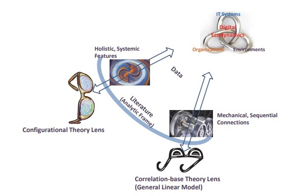
2.2 Configurational Approach vs. Correlational Approach
Configurational approach is sharply different from the correlational approach, which is well explained by the quote “Configurational inquiry represents a holistic stance, an assertion that the parts of a social entity take their meaning from the whole and cannot be understood in isolation. Rather than trying to explain how order is designed into the parts of an organization, configurational theorists try to explain how order emerges from the interaction of those parts as a whole. Social systems are seen as tightly coupled amalgams entangled in bidirectional causal loops. Nonlinearity is acknowledged, so variables found to be causally related in one configuration may be unrelated or even inversely related in another” (Meyer et al. 1993, p. 1178).
Figure 2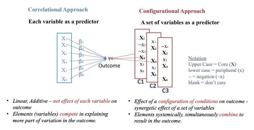
The configurational approach assumes all variables are interdependent with each other and treats a set of variables, not each variable, as a single predictor for the outcome. It does not assume each variable as a sufficient and necessary condition for the outcome, but rather finds which sets of variables sufficiently make the outcome (i.e., a set as a sufficient solution) and which variables are necessary for making the outcome (i.e., a variable as a necessary condition). In Figure 2, there are three sets of variables (i.e., three configurations C1, C2, C3), each of which sufficiently produces the outcome. Furthermore, all configurations include different variables and the role of individual variables vary across the configurations. For example, X1 variable is present in two configurations (C1, C2) while it is absent in other configuration (C3), and it plays a core role in one configuration (C1), but play a peripheral role in other two configurations (C2, C3). As such, the configurational approach allows researchers to explain which variables combine into a configuration to produce an outcome (i.e., conjunction); multiple configurations to achieve the outcome (i.e., equifinality); and the varied roles of each variable across multiple equifinal configurations, causally related in one configuration may be unrelated or even inversely related in another (i.e., asymmetry) (Meyer et al., 1993; Misangyi et al., 2017; Park and Mithas, 2020). Thus, the structure of a configuration exhibiting the outcome may be different from that of a configuration not-exhibiting the outcome. For example, a configuration of high firm performance may have a set of different elements from that of a configuration of low firm performance and even a same element may play different roles between high performance configurations and low performance configurations. Thus, simply increasing or decreasing values of elements in a low performance configuration does not make it as a high performance configuration. These natures of the configurational approach allow us to investigate nonlinear and discontinuous phenomena. Lastly, the diversity of configurations in practice is limited (i.e., limited diversity) due to multiple reasons such as configurations reflecting industry best practices and impossible combinations in reality.
Ⅲ. Qualitative Comparative Analysis (QCA)
3.1 Qualitative Comparative Analysis (QCA)
As a matching method for a configurational approach, qualitative comparative analysis (QCA) was developed by Charles C. Ragin (1987), which is rooted in cross-case comparative analysis to bridge qualitative and quantitative domains in comparative sociology and comparative politics. QCA as a set-theoretic method is built on set-theory and Boolean algebra (Ragin, 2008), and conceptualizes a case (e.g., individual, group, organization, country) as a configuration of relevant elements. For example, in a study of individual health, a unit of analysis is an individual and the study views a case (i.e., individual) as a configuration of multiple factors (e.g., height, weight, gender, race, education, health). Each case has a membership in the set of each factor (e.g., tall group, overweight group, healthy group). QCA uncovers which groups of individuals with specific memberships in these sets of factors have the outcome of interest (e.g., healthy or not): for example, a group of (tall, normal weight, female) individuals exhibiting highly healthy status. Rather than focusing on the correlation or net-effect of each variable (e.g., height or education) on the outcome, QCA finds a configuration of all the factors that produces the outcome. Thus, QCA is best suited to handling the complex interdependencies among the multiple factors and empirically analyzing how they simultaneously combine into multiple configurations to achieve the outcome (Fiss, 2007; Park et al., 2020a; Ragin, 2008).
QCA overcomes mismatch between theory and methods that has plagued earlier configurational research around 1980 ~ 1990, and allows researchers to investigate causality along the three dimensions of complexity: conjunctural, equifinal, and asymmetric (Misangyi et al., 2017; Park and Mithas,2020). Due to such an ability to handle causal complexity, QCA has been widely used by many studies in diverse disciplines (e.g., sociology, strategic management, information systems, finance, marketing, political science). A growing number of studies have employed QCA as their main research approach for deductive theory testing (e.g., Bell et al., 2014) and inductive theory building (e.g., Park et al., 2020b).
This study provides guidelines for researchers in using QCA for theory development and applications of QCA with an empirical example that illustrates how to deploy QCA for theory development. Figure 3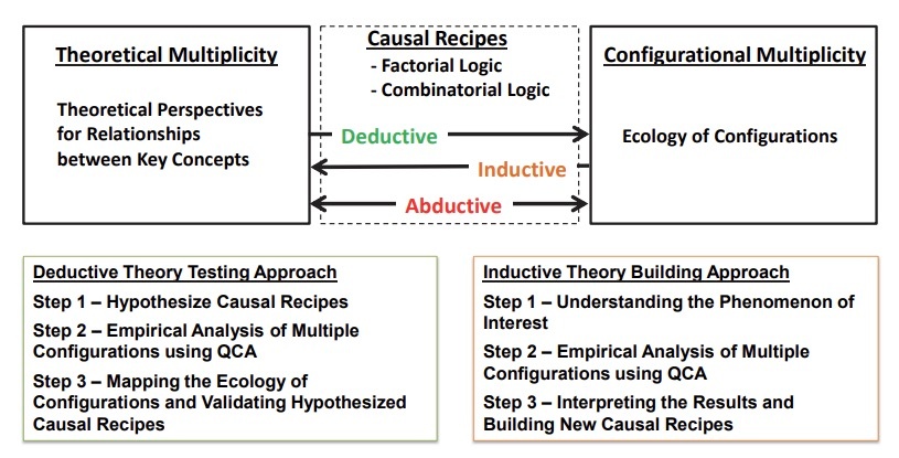
A causal recipe is a formal statement that explains how the causally relevant elements combine into configurations in ways to produce a target outcome, which consists of factorial logic and combinatorial logic. Specifically, a factorial logic describes which elements are important for the outcome of interest to occur and why, as well as which elements are causally not relevant and may be stripped away. On the other hand, the combinatorial logic explains how the different elements of the configuration relate to one another to produce the outcome. Ideally a hypothesis or theoretical proposition is made in the form of causal recipes with factorial and combinatorial logics (Park et al., 2020a).
For the deductive theory testing approach, researchers may first make multiple hypotheses with causal recipes, each hypothesis theoretically predicting which elements combine into a configuration to achieve the outcome and what role each element plays either present/absent or core/peripheral. Hypotheses can also explain the combinatorial logic in terms of complementary, substitutive, or suppressive relationships between elements. Then, by applying QCA to data, researchers find multiple configurations exhibiting the outcome, which in turn empirically validate causal recipes by identifying the existence of corresponding configurations (i.e., hypotheses testing). The inductive theory building is an opposite way, that is, inducing theoretically meaningful causal recipes from empirically observed configurations, which in turn are formed into theoretical propositions.
3.2 QCA Procedure
There are three types of QCA: crisp-set QCA (csQCA), multi-valued QCA (mvQCA), and fuzzy-set QCA (fsQCA) depending on how elements are calibrated, such that csQCA calibrates the original value of element into 1/0, mvQCA into multiple values between 0 and 1, and fsQCA into a continuous value between 0 and 1. Figure 4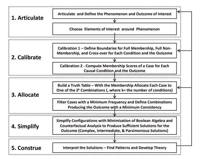
Overall, the research procedure with QCA includes a conceptual development in the front-end, data manipulation with a calibration process, truth-table analysis to find configurations, theoretical interpretation of the results and hypothesis validation or proposition development.
-
“Articulate”: researchers articulate the research topic and specific phenomenon and define the outcome of interest. Then, based on the relevant literature and extant studies with specific theories, they select elements that are relevant to the outcome in the phenomenon, with which a theoretical framework and research model are made from the configurational theory perspective. In QCA, “element, attribute and condition” are used interchangeably presenting the same meaning.
-
“Calibration”: Next step in QCA is to calibrate the elements and outcomes into set-membership scores. Calibration is a process to compute the set-membership scores of each case in causal conditions (e.g., AI investment, top management diversity) and the outcome (e.g., firm performance) by transforming the original value of each variable for a case into a membership score in a specific set. In other words, it defines the extent to which a given case has membership in a specific set/group (e.g., a set of high performing firms, a set of firms with high investment in AI). For csQCA, the calibration process transforms the values of all conditions into either 1 or 0, while for fsQCA it transforms the original values into a fuzzy membership score between 0 and 1, indicating 0 as a full non-membership and 1 as full membership. Ragin’s (2008) direct method of calibration is commonly used, which is based on three qualitative anchors: full membership, full non-membership, and the crossover point of maximum ambiguity regarding membership of a case in the set of interest. A researcher should define these three anchors based on empirical and theoretical knowledge of the context and cases (Fiss, 2011; Park et al., 2020a; Ragin, 2008).
-
“Allocate”: The truth-table algorithm is applied to identify the configurations of causal conditions that sufficiently produce the outcome of interest. As a part of the truth-table algorithm, all cases are allocated into one row in the truth-table. For $k$ elements, there are $2^k$ theoretically possible ideal combinations. In the table, the “Number” column shows the number of cases allocated to each row. Then, we set the minimum acceptable number of cases in a row so that only rows with at least the minimum number of cases are included for subsequent analysis in the truth-table algorithm. The truth-table algorithm then calculates a consistency score that explains how reliably a combination results in the outcome, a measure that is similar to the significance level alpha in regression analysis. For rows that satisfy the frequency threshold, a cutoff for consistency is set so that only combinations with a consistency value greater than the cutoff are considered to reliably result in the outcome.
-
“Simplify”: Next the algorithm reduces the numerous combinations into a smaller set of configurations based on the Boolean algebra and counterfactual analysis (Fiss, 2007; Ragin, 2008). With the updated truth-table, using Boolean algebra, the algorithm reduces the numerous combinations into a smaller number of more parsimonious solutions (Ragin, 2008). For example, if a combination $A \& B$ and $\sim A \& B$ result in the desirable outcome, then regardless of whether $A$ is present or absent ($A \& B + \sim A \& B = B$), the outcome still occurs, where $\&$ means logical AND, $+$ means OR, and $\sim$ means a “negation.” Thus, $A$ does not matter and $B$ alone becomes a sufficient solution for achieving the outcome. Next, the truth-table algorithm utilizes counterfactual analysis to handle the rows without empirical cases (i.e., logical remainders) and to further minimize the number of causal conditions in a configuration. By using “easy” counterfactuals, QCA deals with an empirically unobserved combination by adding a condition known to produce the outcome to a combination. Furthermore, with “difficult” counterfactuals, it deals with an empirically unobserved combination by removing a redundant condition from a combination (Ragin 2008, p.162). QCA generates the most parsimonious solution by applying both easy and difficult counterfactuals and the elements in this result are considered to be core conditions that have a stronger causal relationship with the outcomes (Fiss, 2011). By applying only easy counterfactuals,QCA creates intermediate solutions that include peripheral conditions that have weaker causal relationships with an outcome as well as core conditions. Thus, with intermediate solutions, we can explain which conditions play a core role or a peripheral role in producing the outcome of interest. Furthermore, in addition to multiple configurations that sufficiently produce the outcome, QCA allows us to find necessary conditions for the outcome. A necessary condition is a superset of the outcome, meaning that the outcome could not be achieved without having the necessary condition.
-
“Construe”: As a final step in QCA, researchers should interpret the results theoretically (i.e., configurations that sufficiently produce the outcome, and necessary conditions). By comparing similarities and differences across configurations, researchers can uncover patterns regarding combinatorial and factorial logics, which in turn enable us to test the proposed hypotheses or to build propositions. As aforementioned, a factorial logic describes which elements are important or less relevant for the outcome of interest to occur and why, while the combinatorial logic explains how the different elements of the configuration relate to one another to produce the outcome. Hypothesis or theoretical proposition is made in the form of causal recipes consisting of factorial and combinatorial logics (Park et al., 2020a).
Ⅳ. Illustrative Example
In the following, an illustrative example is provided to show how to apply QCA through the suggested steps. Specifically, it illustrates a theory building with an abductive configurational approach, explicating how QCA enables researchers to build a unified theory that can address the issues from theoretical multiplicity (Lee et al., 2019). This example is excerpted directly from the study by Lee et al. (2019), which suggests holistic archetypes of Information Technology (IT) outsourcing strategy that overcomes the inconsistent and fragmented findings in the extant studies of IT outsourcing projects built on different theories. So, more detailed explanation of theoretical development, data collection and methods can be found in Lee et al. (2019).
Articulations: IT outsourcing projects are well-known for the complexity and causal ambiguity of coordinating diverse outsourcing activities, particularly in the relationships between a focal firm and its outsourcing vendors (Ravindran et al. 2015). To achieve the success of IT outsourcing project, a firm should effectively tackle the complexity of ininter-organizational relationships (IOR) such as information asymmetry and conflict of interest with its outsourcing vendors. Extant studies have revealed multiple equally viable key mechanisms that enable firms to effectively manage IOR complexity and achieve outsourcing project success, including cost efficient transactions reflected in transaction cost economics theory (TCET), control of critical resource dependency in resource dependency theory (RDT), and reciprocal relationship building in social exchange theory (SET). Extant studies based on these theories have greatly contributed to our understanding of the IOR between a client and its vendors, especially in terms of four key relationship elements: degree of IT outsourcing (Dibbern et al., 2012; Lacity and Willcocks, 1996), relationship type (Gopal and Koka, 2012; Handley and Angst, 2015), period of the IT outsourcing contract (Goo et al., 2007; Ravindran et al., 2015), and the number of vendors (Poston et al., 2009; Su and Levina, 2011). However, extant studies adopting these theories have made fragmented, incomplete, and contradictory findings by focusing on the net effect of individual elements and paid little attention to their combined interdependent effects on IT outsourcing success, leaving managers uncertain about effective management of the complex interfirm relationships and researchers unclear about which theories are most relevant in studying IT outsourcing projects. For example, extant studies based on SET have suggested long-term reciprocal partnerships so that a firm shares risks and strategic benefits with their vendors (e.g., Ravindran et al., 2015), while studies with TCET have suggested a short-term fee-for-service contract as an effective pathway to achieving cost efficiency (e.g., Lacity and Willcocks, 1996) whereas RDT studies have highlighted a strategic advantage by minimizing a firm’s resource dependency on others with a selective outsourcing, buy-in contract or by controlling key resources via cooperative alliances with its vendors (e.g., Ulrich and Barney, 1984). Furthermore, even studies adopting the same theory have often reported inconsistent findings in terms of the four IOR elements.
Degree of IT outsourcing is defined as the extent to which a firm outsources its functions and related business (Dibbern et al., 2012; Lacity and Willcocks, 1996). In past work, scholars have measured the degree of IT outsourcing as the percentage of the total IT budget spent for outsourcing, often categorized into three groups - minimal outsourcing, selective outsourcing, and total outsourcing. Relationship type is defined as a kind of outsourcing contract between a focal firm and its outsourcing vendors (Gopal and Koka, 2012; Handley and Angst, 2015), including fee-for-service, partnership, and buy-in. With a fee-for-service contract, a firm pays a fee to a service vendor in exchange for the management and delivery of specified IT products or services. The partnership contract is a collaborative relationship that involves resources from both a client firm and its vendors to increase mutual benefits for both parties. With a buy-in contract, a firm purchases vendor resources and internally manages these purchased resources itself to minimize its resource dependency on vendors. Period of outsourcing is defined as the duration of an outsourcing contract (Goo et al., 2007; Ravindran et al., 2015). Some studies codify period as short-term, medium-term, and long-term instead of a temporal, continuous metric like years. The number of outsourcing vendors is the actual number of external vendors involved in an IT outsourcing project (Poston et al., 2009; Su and Levina, 2011). The overarching theoretical framework that integrates the three dominant theories of the inter-organizational relationships is built on the systems contingency fit approach in a way to uncover consistent patterns among IOR elements under specific organizational and environmental contexts in achieving the success of IT outsourcing project (Lee et al., 2019: p. 1207).
Calibration
This example uses survey data collected from 235 firms listed on the Korea Exchange, which had major IT outsourcing projects. To apply fsQCA, this study uses the direct method of calibration that transforms an original value to a fuzzy membership score based on three qualitative anchors: full membership, full non-membership, and the crossover. A summary of three anchors for all conditions and the outcome is given in Table 1
Table 1 Summary of calibration of causal conditions and outcome
| Conditions and outcome | Coding and Calibration |
|---|---|
| Outsourcing success | Strategic Benefits (sum of five items) - Full membership anchor = 30 - Cross-over anchor = 20 - Full non-membership anchor = 10 *Each item is measured by 7-point Likert scale (7 = very successful, 4 = neutral (neither in nor out), 1 = not successful). |
| Degree of IT outsourcing | For total outsourcing - Full membership anchor = more than 80% of IT budget - Cross-over anchor = 50% of IT budget - Full non-membership anchor = less than 20% of IT budget |
| Period of outsourcing | For long-term contract (years) - Full membership anchor = 8 - Cross-over anchor = 5 - Full non-membership anchor = 2 |
| Number of outsourcing vendors | - 1 when multi-vendor (more than one vendor), 0 for single vender |
| Relationship type | - Fee-for-service contract = 1 when relationship type is either standard or detailed or loose or mixed contract, otherwise 0: - Partnership contract = 1 for partnership type, otherwise 0. - Buy-in contract = 1 for buy-in type, otherwise 0. |
| Outsourced IT type | - 1 = IT application outsourcing, 0 = IT Infrastructure outsourcing |
| Firm size | For large firms (based on the number of employees) - Full membership anchor = 5000 - Cross-over anchor = 1000 - Full non-membership anchor = 200 |
Allocate
Based on the calibrated memberships, each case is allocated into one of the rows in a truth-table that displays all possible combinations of the elements made with logical AND operation, each row corresponding to one combination. For example, a not-large firm with not-total outsourcing, fee for service and long-term contract with one vendor is allocated to the first row in the truth-table shown in Table 2
Table 2 Truth-table – combinations of outsourcing elements for economic benefits
| Degree of IT out. (Total) | Relationship type: Fee for svc | Relationship type: Partnership | Relationship type: Buyin | Period of out. (Long-term) | Num. of out. vendors (Multi) | Out. IT Type (App 1, Infra 0) | Firm size (Large) | Num. | High econ. benefits | Raw consistency | PRI Consistency |
|---|---|---|---|---|---|---|---|---|---|---|---|
| 0 | 1 | 0 | 0 | 1 | 0 | 0 | 0 | 6 | 1 | 1.00 | 1.00 |
| 1 | 1 | 0 | 0 | 1 | 1 | 0 | 0 | 8 | 1 | 1.00 | 1.00 |
| 1 | 1 | 0 | 0 | 1 | 1 | 1 | 0 | 8 | 1 | 1.00 | 1.00 |
| 0 | 1 | 0 | 0 | 0 | 0 | 0 | 0 | 7 | 1 | 0.97 | 0.95 |
| 1 | 1 | 0 | 0 | 1 | 1 | 0 | 1 | 9 | 1 | 0.97 | 0.95 |
| 1 | 0 | 1 | 0 | 1 | 1 | 1 | 1 | 8 | 1 | 0.95 | 0.90 |
| 1 | 0 | 1 | 0 | 1 | 0 | 0 | 1 | 8 | 1 | 0.94 | 0.90 |
| 1 | 0 | 1 | 0 | 1 | 1 | 0 | 1 | 9 | 1 | 0.94 | 0.91 |
| 1 | 0 | 1 | 0 | 1 | 0 | 0 | 0 | 7 | 1 | 0.93 | 0.88 |
| 1 | 0 | 1 | 0 | 1 | 0 | 1 | 1 | 7 | 1 | 0.93 | 0.88 |
| 0 | 1 | 0 | 0 | 0 | 0 | 0 | 1 | 8 | 1 | 0.92 | 0.85 |
| 1 | 0 | 1 | 0 | 1 | 0 | 1 | 0 | 10 | 1 | 0.91 | 0.89 |
| 0 | 1 | 0 | 0 | 1 | 0 | 1 | 1 | 5 | 1 | 0.91 | 0.80 |
| 0 | 1 | 0 | 0 | 0 | 0 | 1 | 1 | 5 | 1 | 0.91 | 0.81 |
| 1 | 0 | 1 | 0 | 1 | 1 | 0 | 0 | 10 | 1 | 0.89 | 0.84 |
| 1 | 0 | 1 | 0 | 1 | 1 | 1 | 0 | 14 | 1 | 0.86 | 0.79 |
| 0 | 0 | 0 | 1 | 0 | 0 | 0 | 1 | 24 | 0 | 0.84 | 0.73 |
| 0 | 0 | 0 | 1 | 0 | 0 | 1 | 1 | 12 | 0 | 0.84 | 0.72 |
| 0 | 0 | 0 | 1 | 0 | 0 | 0 | 0 | 8 | 0 | 0.83 | 0.59 |
| 0 | 0 | 0 | 1 | 0 | 0 | 1 | 0 | 8 | 0 | 0.78 | 0.55 |
Next, to determine which combination consistently becomes a sufficient solution for the outcome, it uses a measure of consistency, “the degree to which the cases sharing a given combination of conditions (i.e., a row in the Truth-Table) agree in displaying the outcome in question” (Ragin 2008, p. 44), similar to the significance level alpha in regression analysis. In this example, it shows whether firms sharing a same set of outsourcing elements consistently result in outsourcing success. In fsQCA, there are two types of consistency: raw consistency, which is calculated by giving credit for “near misses” and penalties for large inconsistencies and PRI consistency (a proportional reduction for inconsistency), an alternate measure of consistency that in addition eliminates the influence of cases that have simultaneous membership in both the outcome and its complement (i.e. $y$ and $\sim y$). This example study sets 0.85 as cutoff for raw consistency and 0.75 for PRI consistency, meaning that only combinations with a raw consistency of at least 0.85 and a PRI consistency of at least 0.75 are considered to be reliably resulting in the outcomes. In the truth-table, outsourcing performance (i.e., economic benefits) has a value 1 for the combinations that satisfy this consistency cutoff, otherwise 0. Thus, not a single or individual elements but a combination of all elements becomes one predictor for the outcome. The higher consistency thresholds the more consistent solution. Ragin (2008) suggests 0.75 as the minimum threshold for raw consistency, but there is no single standardized number for consistency threshold accepted in the QCA literature. Extant QCA studies in general use at least 0.8 as a minimum threshold for raw consistency and 0.7 for PRI consistency. But, some studies use higher or lower thresholds depending on data and contexts. Thus, it is important to check the robustness of the results and additional sensitive analysis is mostly required. For example, in this example a sensitivity analysis can be done with different frequency cutoffs (e.g., 3, 7) and different raw/PRI consistency thresholds (e.g., 0.8, 0.7) to check whether the key results would sustain possibly with minor change or radically change.
Simplify
With the minimization of Boolean algebra, the truth-table algorithm reduces the rows in the updated truth-table and makes a complex solution. Then, with counterfactual analysis the algorithm further minimizes combinations of conditions. With easy counterfactual analysis, intermediate solution is made, and with both easy and difficulty counterfactual analysis parsimonious solution is made. Conditions in the parsimonious solution are core elements in configurations, while other elements belonging only in the intermediate solution are peripheral.
Bold font elements in intermediate solutions represent parsimonious solutions, meaning they are core elements that have a stronger causal relationship with the outcomes. * P = Partnership, B = Buy-In, F = Fee for service, Size = (Large) firm size, Total = Total Outsourcing, Long = Long-term contract, Infra = IT Infrastructure (outsourced), App = IT Application (outsourced), Single/Multi vendors element (Fiss, 2011). The results of simplification process with the truth-table algorithm are presented in Table 3
Table 3 fsQCA results: Configurations sufficiently producing the outcome
| Parsimonious Solution | Intermediate Solution |
|---|---|
| $\sim$B $\rightarrow$ economic benefits | Total&($\sim$B&P&$\sim$F)&Long (20 cases) + Total&($\sim$B&$\sim$P&F)&Long&Multi&Infra (17 cases) + Total&($\sim$B&$\sim$P&F)&Long&Multi&$\sim$Size (16 cases) + $\sim$Total&($\sim$B&$\sim$P&F)&Single&Infra&$\sim$Size (13 cases) + $\sim$Total&($\sim$B&$\sim$P&F)&$\sim$Long&Single&Infra (15 cases) + $\sim$Total&($\sim$B&$\sim$P&F)&Single&App&Size (10 cases) + $\sim$Total&($\sim$B&$\sim$P&F)&$\sim$Long&Single&Size (13 cases) $\rightarrow$ economic benefits |
Figure 5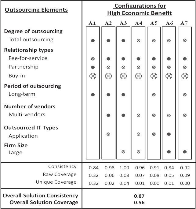
^ Full circles indicate the presence of a condition, and crossed-out circles indicate its absence. Large circles indicate core conditions; Small ones, peripheral conditions. Blank spaces indicate “don’t care” situations where the element may be either present or absent. ^* For clarification, absence of total outsourcing (crossed-out circle) means selective outsourcing, absence of application = IT infrastructure, absence of multi-vendors = single vendor, absence of large = not large (small or medium) size firm, and absence of long-term = short or medium term. For the relationship type, only one of the three types can be present.
Raw coverage is the extent to which each configuration covers the cases of outcome, a measure similar to explained variance ($R^2$) in correlational analysis. Unique coverage of a configuration is the portion of coverage that is explained by the configuration, without its overlapping with other configurations. Thus, coverage shows an empirical relevance and effectiveness of the configuration for producing the outcome, although a higher coverage does not necessarily mean higher theoretical importance (Ragin 2008, p. 44). In these equifinal configurations, the coverage of configuration A1, “total outsourcing with long-term partnership,” is the largest, meaning that it is empirically the most relevant and effective in achieving both economic benefits and strategic benefits in IT outsourcing (Ragin 2008, p. 44).
In addition to the sufficient solution of configurations, a necessary condition test was done for all conditions and their negations. But there was no condition of which consistency measure is greater than 0.9, the minimum consistency to be qualified as a relevant necessary condition (Ragin, 2008).
Construe
As a final step in QCA, researchers should interpret the results theoretically based on extant studies from the dominant theories and suggest theoretical propositions. As an illustrative purpose, I explain here one theoretical proposition built from the findings and theoretical interpretations. More propositions with detailed theoretical interpretation of the findings can be found in Lee et al. (2019).
Figure 6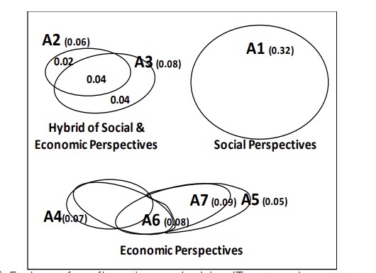
Based on the theoretical distinction, we can interpret each group separately from its theoretical perspective and make a proposition. For example, configuration A1 shows that IT outsourcing project with “total outsourcing with a long-term partnership relation” can achieve high economic benefits. This pattern reflects the social perspective of both SET and RDT. The stream of research based on SET has historically emphasized the importance of long-term partnerships between a focal firm and its outsourcing vendors (Ravindran et al., 2015). While some RDT studies view partnerships as a way to stabilize its resource dependency on others, a firm, in order to be successful, needs to keep control over critical resources in business environments by developing cooperative relationships such as long-term strategic alliances and joint ventures with its outsourcing vendors (Pfeffer and Salancik, 1978; Ulrich and Barney, 1984). A1 also clearly shows “long-term, partnership contracts with total outsourcing” achieve the outcome regardless of the number of outsourcing vendors, outsourced IT types, and firm size. This particular pattern enables us to explicate the role of all four IOR elements and suggest a more holistic, specific underlying mechanism effective over diverse contexts, thus sharpening and expanding the core mechanisms of both SET and RDT. Based on the finding and its theoretical interpretation, a proposition is posited as follows:
Proposition 1. Social Archetype of IT Outsourcing Strategy: Total outsourcing with long-term partnership relations can achieve high economic benefits in all types of IT outsourcing projects regardless of vendor number, firm size and IT types.
For the other two groups of economic theoretical perspective (A4~A6) and hybrid theoretical perspective (A2, 3), theoretical interpretation and proposition development can be found in Lee et al. (2019).
Ⅴ. Conclusion and Implications
In the pervasively digitalized world, digital technologies are increasingly fused and entangled with business processes, structures, people, and things, thus creating novel value-creation mechanisms that are more complex. Such complex digital phenomena require organizations to shift the way to create innovations and business values from individual resources to the holistic system in which all elements are interdependent with each other.
I would like to emphasize that this study does not argue that a configuration approach with QCA is superior to a correlation-based approach in theory building, but rather can complement the correlation-based variance theory approach which has been dominant for last decades in the management and IS research. This study explained that the configurational research approach provides a new alternative way to theory building, especially by explicating a specific way to apply a set-theoretic method QCA to build a new theory of conjunctural, equifinal, and asymmetrical causality in a complex business phenomenon, in which digital elements are intertwined with organizational elements to produce the outcomes of interest under varying environments. Thus, this study helps researchers understand the unique problems of causal complexity and select a most appropriate research approach and method to build a target theory. I hope that the detailed guidelines for applying QCA along with an illustrative example would be useful for researchers to learn and use QCA to build a novel theory with configurational causal recipes.
Figure 2 Configurational vs. Correlational Approach
| Correlational Approach | Configurational Approach |
|---|---|
| Each variable as a predictor | A set of variables as a predictor |
| $X_1 \xrightarrow{\beta_1} Y$ | C1: $X_1, \sim X_2, \sim X_3, X_4, x_5, x_6$ |
| $X_2 \xrightarrow{\beta_2} Y$ | C2: $x_1, X_2, X_4, x_5, X_6$ |
| $X_3 \xrightarrow{\beta_3} Y$ | C3: $\sim x_1, X_2, X_3, X_4, X_6$ |
| $X_4 \xrightarrow{\beta_4} Y$ | Notation |
| $X_5 \xrightarrow{\beta_5} Y$ | Upper Case = Core ($X$) |
| $X_6 \xrightarrow{\beta_6} Y$ | lower case = peripheral ($x$) |
| $\sim$ = negation ($\sim x$) | |
| blank = don't care | |
| • Linear, Additive – net effect of each variable on outcome | • Effect of a configuration of conditions on outcome - synergetic effect of a set of variables |
| • Elements (variables) compete in explaining more part of variation in the outcome. | • Elements systemically, simultaneously combine to result in the outcome. |